Theoretical Improvements - Mixing Liquids: Molecular Solutions - Liquid-State Physical Chemistry: Fundamentals, Modeling, and Applications (2013)

Liquid-State Physical Chemistry: Fundamentals, Modeling, and Applications (2013)

11. Mixing Liquids: Molecular Solutions

11.9. Theoretical Improvements*

Next, let us turn to attempts to improve the local configuration. In the ideal solution model it is assumed that the distribution of the components 1 and 2 is random. The same is assumed for the regular solution model, although preferential energetic interactions are also assumed. This state of affairs represents, at least, an inconsistency.

In order to improve, let us recapitulate the regular solution model in slightly different words. Consider the interchange 1–1 + 2–2 → 1–2 + 2–1 on a lattice with coordination number z, to which we attributed an interchange energy 2w. We have a total of ½zN pairs of nearest-neighbor bonds, irrespective of their type. We now define zX to be the total number of 1–2 pairs for a particular distribution. Since the number of neighbors of type 1 molecules that are not of type 2 is z(N₁ − X), the number of 1–1 pairs is ½z(N₁ − X). Similarly, the total number of 2–2 pairs is ½z(N₂ − X), respectively. The problem is now to determine the average value of X.

Assuming a completely random distribution over sites, the relative probability of a 1–1 and a 2–2 pair is equal to the probability of a 1–2 and a 2–1 pair. Therefore

(11.132)

This immediately leads to the solution , and from this all previous results follow. In particular, the configurational interaction energy

(11.133) 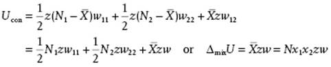c11-math-0133

This approximation has different names in different fields and we designate it here (in accordance with Guggenheim) as the zeroth approximation. It is also known as the mean field approximation.

The basic tenet here is the independent distribution of single molecules over sites, in spite of their nonzero interchange energy w. Systematic improvement is possible by considering the independent distribution of pairs of molecules (first approximation), of triplets of molecules (second approximation), and so on, taking into account the interchange energy within a multiplet. Of course, the independent pair model is also deficit because a certain local configuration cannot be realized by adding independent pairs. For example, in a four coordinated lattice the first three pairs can be chosen independently, but the fourth cannot. A similar statement can be made also for the higher approximations. However, we might expect to obtain a better description as with the independent distribution of single molecules. The independent distribution of pairs, as discussed in Appendix C [9, 15], provides some improvement (and is an interesting approach as such). The expression for Δ_mixG_m (or Δ_mixF_m) is somewhat complex, and for details we refer to Appendix C. For the critical temperature the simple expression zw/kT_cri = z ln [z/(z − 2)] results.

Before we discuss the improvement in numerical results, we first note that the scheme 1–1 + 2–2 → 1–2 + 2–1 strongly resembles the scheme for a chemical reaction. Even the equation X² = (N₁ − X) (N₂ − X) resembles a reaction equilibrium expression. This led Guggenheim [16] to introduce the so-called quasi-chemical approximation by postulating that the equation X² = (N₁ − X) (N₂ − X) must be modified heuristically to include the interchange energy so that it becomes X² = (N₁ − X) (N₂ − X) exp(−2βw). In this way, the analogy with a chemical reaction is more or less complete. Later, this approach was shown to be completely equivalent to the independent pair distribution approach, which we have labeled here as the first approximation, and this approach has been used ever since for many applications. Obviously, the use of triplets and quadruplets instead of pairs improves the estimate; however, the details become rapidly complex and we refrain from discussing details, referring the interested reader to Guggenheim [17, 18].

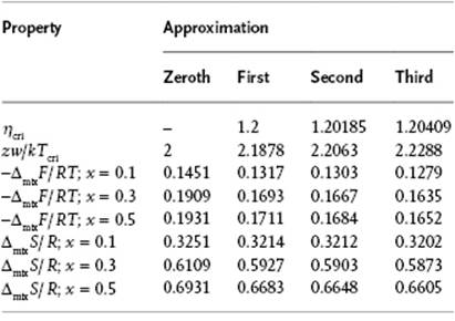
Let us now quote a few results of the zeroth, first, and higher approximations [17, 18] to see what the improvements are as compared to the zeroth approximation. From Table 11.6 it is clear that for the critical temperature T_cri and the Helmholtz energy of mixing Δ_mixF, the first approximation is an improvement over the zeroth, but that higher approximations do not yield a significant improvement. A similar observation can be made for the vapor pressure (not shown). For the entropy of mixing Δ_mixS, the values for the higher approximations are close to that of the zeroth. In conclusion, when using this combinatorial approach for molecular solutions, in all cases the first approximation is sufficiently accurate and, although this is a conceptual improvement, in many cases even the zeroth approximation is sufficient, in contrast to the case of polymeric solutions (see Chapter 13). Finally, we note also that the effect of next-nearest-neighbor interactions has been assessed. It appears that this effect is much smaller than the differences between the zeroth and first approximation, and therefore can be entirely neglected.

Table 11.6 Critical temperature, Helmholtz energy and entropy in several approximations for close-packed lattice with z = 12.

c11-tbl-0006

In spite of the relative simplicity of the zeroth order model, an analytical solution is known so far only for 2D lattices. For a square 2D lattice with z = 4 this solution reads [19] sinh (zw/4kT_cri) = 1, which gives zw/kT_cri = 3.526. For comparison, we recall that in the zeroth approximation zw/kT_cri = 2.0, whilst for the first approximation zw/kT_cri = z ln [z/(z − 2)] = 2.773 was derived. Hence, in conclusion, although the first approximation constitutes a conceptual and numerical improvement as compared to the zeroth approximation, the difference with the exact solution is still significant. One expects this also to be true in 3D, and a numerical evaluation of the 3D problem indeed showed this to be true (see Chapter 16 and Appendix C).

Notes

1) Although we use Z_m for a molar quantity, often the subscript m is left out if the meaning is clear from the context. Moreover, while for an arbitrary amount n_α of component α the expression Z = n_αZ_α holds exactly for any extensive quantity Z, it is sometimes approximated by , in particular for the volume V. Note that for a pure component, .

2) Note that the partial pressure is not a partial quantity as defined here. This is unfortunate but the designation is conventional.

3) Note that for all i–j interactions the parameter w_ij = −|w_ij| < 0.

4) Bernal estimated that for more or less spherical molecules the ratio of molecular volumes must be between 1 and 2, equivalent to a diameter ratio of 1.26 (see Ref. [24]).

5) Note that in this model for the pure component F_α = U_α − TS_α = U_α.

6) We recall that for all i–j interactions the parameter w_ij = −|w_ij| < 0.

7) The reference value depends on the choice of the composition parameter used. A different value is thus used for the mole fraction, molarity or molality scale. As long as one adheres to a particular choice, this provides no problem.

8) Here we use u for the pair potential energy since ϕ is (conventionally) used for the volume fraction.

9) The partial volume V_α is often approximated by the molar volume of the pure component .

References

1 See Pitzer (1995).

2 Guggenheim, E.A. (1937) Trans. Faraday Soc., 33, 151.

3 Adcock, D.S. and McGlashan, M.L. (1954) Proc. Roy. Soc., A226, 266. See also Guggenheim (1967), p. 199.

4 Hildebrand, J.L. and Wood, G.E. (1933) J. Chem. Phys., 1, 817. See also Hildebrand and Scott (1962).

5 Hildebrand, J.H. (1919) J. Am. Chem. Soc., 41, 1067. See also Hildebrand and Scott (1962).

6 Reed, T.M., III (1955) J. Phys. Chem. Soc., 59, 429.

7 (a) Henderson, D. and Leonard, P.J. (1971) Proc. Natl Acad. Sci. USA, 68, 632; (b) Lee, L.L. (1988) Molecular Thermodynamics of Nonideal Fluids, Butterworth, Boston.

8 (a) Redlich, O., Kister, A.T., and Turnquist, C.E. (1952) Chem. Eng. Progr. Symp. Ser. 2, 48, 49; (b) However, the expansion was already used by Guggenheim, E.A. (1937) Trans. Faraday Soc., 33, 151.

9 See Guggenheim (1952).

10 (a) Van Laar, J.J. (1910) Z. Phys. Chem., 72, 723; (b) Van Laar, J.J. (1913) Z. Phys. Chem., 89, 599; (c) See also: Van Laar, J.J. (1906) Sechs Vorträge űber das thermodynamische Potential. Vieweg Verlag, Brunswick, Germany.

11 Scatchard, G. (1931) Chem. Rev., 8, 321.

12 Prausnitz, J.M., Lichtenthaler, R.N., and de Azevedo, E.G. (1986) Molecular Thermodynamics of Fluid Phase Equilibria, Prentice-Hall, Englewood Cliffs, NJ, Ch. 6.

13 Wilson, G.M. (1964) J. Am. Chem. Soc., 86, 127.

14 Ohe, S. (1989) Vapor-liquid Equilibrium Data, Elsevier, Amsterdam.

15 See Lucas (2007).

16 (a) Guggenheim, E.A. (1935) Proc. Roy. Soc., A148, 304; (b) Rushbrooke, G.S. (1938) Proc. Roy. Soc., A166, 296.

17 Guggenheim, E.A. (1952) Applications of Statistical Mechanics, Clarendon, Oxford.

18 Guggenheim, E.A. (1966) Applications of Statistical Mechanics, Clarendon, Oxford.

19 Onsager, L. (1944) Phys. Rev., 65, 117.

20 von Zawidski, J. (1900) Z. Phys. Chem., 35, 129.

21 See Smith et al. (2005).

22 Silbey, R.J. and Albert, R.A. (2001) Physical Chemistry, 3rd edn, J. Wiley & Sons Ltd, New York.

23 Atkins, P.W. (2002) Physical Chemistry, 7th edn, Oxford University Press.

24 Fowler, R.H. and Guggenheim, E.A. (1939) Statistical Thermodynamics, Cambridge University Press, London, p. 351.