Liquid-State Physical Chemistry: Fundamentals, Modeling, and Applications (2013)

13.2. Real Chains in Solution

In the previous paragraph we discussed mainly chains in the absence intermolecular interactions, that is, ideal chains. Furthermore, we indicated that the balance between segment–segment interactions on the one hand and segment–solvent interactions on the other hand determine the behavior of polymer in solution. In this section, we elaborate on the latter topic using the equivalent chain with n segments of length b, inspired by the treatment as given by Rubinstein and Colby [2].

Let us thus be somewhat more precise about the interactions. The effective segment–segment interactions are obviously dependent on the solvent used, and are often called excluded volume interactions. If the effective interaction energy between segments is Φ(r), the statistics are determined by the Boltzmann factor exp(−βΦ); however, if we have no effective interaction, then Φ(r) = 0 so that exp(−βΦ) = 1. The net result is thus conveniently described, using the Mayer factor f(r) = exp(−βΦ) − 1, by the integral

(13.11)

representing the excluded volume υ. If υ < 0, the net interaction is attractive, while for υ > 0 the net interaction is repulsive. If there is hardly any difference between segment–segment and segment–solvent interactions, the solvent is denoted as an athermal solvent. At low concentration, the Helmholtz energy F can be described by a virial expression in terms of the segment concentration. We recall that such an expansion for F containing an ideal and an interaction part reads

(13.12)

where υ represents the two-segment contribution (the excluded volume) and ω the three-segment interaction.

The two-segment and three-segment interactions also depend on the shape of the segments. So far, we have assumed spherical segments, but it is somewhat more realistic to use cylindrical segments with length b and (somewhat) smaller diameter d. Flexible polymers typically have a b/d ratio in the range 2 to 3, whereas for stiffer polymers the value is somewhat larger. For athermal spherical segments with diameter d, we have υ_s ∼ d³ and ω_s ∼ d⁶. However, the interaction must not change if we redefine our segment. A chain with n_s spherical segments of diameter d can also be considered as a chain of n_c = n_sd/b cylindrical segments of diameter d and length b. So, υ_sn_s² = υ_cn_c² and ω_sn_s³ = ω_cn_c³. For the cylindrical segments we therefore obtain⁴⁾

(13.13)

The ratio of excluded volume υ_c ∼ b²d over occupied volume υ₀ ∼ bd² is b/d, and it will be clear that the excluded volume depends strongly on the shape of the segment. Note that by taking b = d we regain the expression appropriate for spherical segments.

Using this image we can distinguish between several types of solvent:

· Athermal solvents. For these solvents the segment–segment interactions equal the segment–solvent interactions, so that only the core repulsions between the segments control the interaction. Hence, υ ≅ b²d.

· Good solvents. In these solvents the segment–segment attraction is somewhat larger than the solvent–segment attraction. Consequently, 0 < υ < b²d.

· Theta solvents. At a certain temperature (the θ-temperature) the segment attractions cancel the core repulsions. This leads to υ ≅ 0. At T = θ the chains have near-ideal conformations.

· Poor solvents. For T < θ, the attractive interactions between the segments are relatively strong so that the segments clog together. The excluded volume is negative, and we have −b²d < υ < 0.

· Non-solvents. For strong segment–segment attraction we obtain the limit of a poor solvent, that is, the non-solvent. In this case, υ ≅ −b²d.

Our task is now to provide a model for this behavior.

Flory developed a relatively simple theory with energetic and entropic contributions to describe a polymer solution using a good solvent. For his model, Flory assumed that the n segments are homogeneously distributed without any correlation in a sphere of radius R > R₀ = n^1/2b. The probability of finding a second segment in an excluded volume υ of a given segment equals the product of υ and the number density n/R³, that is, υn/R³. Because the energy increase of an excluded volume interaction is kT per exclusion, we have for the n segments in the chain U ∼ kTυn²/R³. The entropy is estimated by the Gaussian chain estimate −TS ∼ kTR²/nb². In total, we thus have

(13.14)

From ∂F/∂R = 0 we obtain for the Flory chain R_F = υ^1/5n^3/5b^2/5, to be compared with the Gaussian chain result R = R₀ = n^1/2b. The relative size of the Flory chain with respect to the Gaussian chain is therefore R_F/R₀ ∼ υ^1/5n^3/5b^2/5/n^1/2b ∼ (υn^1/2/b³)^1/5, and chains only swell when the chain interaction parameter z = υn^1/2/b³ is positive and sufficiently large. For z < 0, the chain remains nearly ideal.

It appears that the Flory theory describes experiments rather well, but this is the result of some canceling errors (see, for example, Ref. [2]). The description as given here is akin to the self-avoiding random walk (SAW) model in which one stipulates that the freely jointed chain cannot intersect itself, contrary to the Gaussian chain where all conformations are possible. More sophisticated theory yields for the exponent ν = 0.588 instead of ν = 3/5.

The differences between the Gaussian and Flory chain become rather clear if we compare their behaviors under tension. To that purpose, we note that most of the entropy is the result of conformational freedom at the smallest length scale. Hence, we use the image that a chain containing n segments is constructed from smaller sections of size ξ, each containing g segments. Upon applying tension to the chain, each section – often referred to as a tension blob – is essentially unperturbed, but the blob more or less moves as a whole under the applied tension. Therefore, one degree of freedom is restricted, increasing the Helmholtz energy by kT. The result for F thus becomes F ∼ kTn/g∼ kTL²/nb², in agreement with Eq. (13.10). The physical interpretation of a blob is that ξ is the length for which the external tension changes the overall conformation from almost undeformed for length scales r < ξ to extended for length scales r > ξ.

For the size of the blob ξ and the contour length L we have, respectively,

(13.15)

Solving for ξ and g we obtain

(13.16)

For the Gaussian and Flory chain we have, respectively,

(13.17)

Furthermore, we assume that a subsection of size r of the chain scales similarly, that is

(13.18)

so that for the blob size we obtain

(13.19)

The end-to-end distances for the two chains, here again labeled by X, are

(13.20)

Solving for ξ we obtain

(13.21)

and calculating the Helmholtz energy, recalling that the energy for stretching is kT per blob, the result becomes

(13.22)

The forces for stretching are, as usual, given by f = ∂F/∂X and become

(13.23)

or, equivalently,

(13.24)

For both types of chains the stretching energy is kT per segment when the chain is nearly fully stretched, but, although the force increases faster with X for the Flory chain, it is always smaller than for the ideal chain. For both chains the number of available conformations decreases when stretched, but the Flory chain has fewer conformations to lose, which results in a smaller force.

13.2.1 Temperature Effects

We will consider thermal effects also using a scaling approach. Since we encoun­­ter both attractive and repulsive excluded volume interactions, we use |υ| in definitions and indicate the sign explicitly where needed. Similar to stretching, we assume that a thermal length scale exists, the thermal blob size ξ_T, for which the excluded volume interactions are smaller than the thermal energy kT, if the length scale r < ξ_T. The conformations of the thermal blob are then nearly ideal and if the blob contains g_T segments, we have

(13.25)

The size of the blob ξ_T can be estimated by equating the excluded volume interaction kT|υ|g_T²/ξ_T³ for a single blob with the thermal energy kT, that is

(13.26)

Combining Eq. (13.25) and (13.26) we obtain

(13.27)

The blob size is the value where excluded volume interactions become important. For υ ∼ b³, ξ_T ∼ b, the blob has the size of a segment and is fully swollen in an athermal solvent. For υ ∼ −b³, again ξ_T ∼ b and the chain is fully collapsed in a non-solvent. For |υ| < b³n^−1/2, ξ_T > R₀, and the chain behaves as nearly ideal. Finally, for b³n^−1/2 < |υ| < b³, ξ_T is between segment and chain size with moderate swelling in a good solvent (υ > 0) or moderate collapse in a poor solvent (υ < 0).

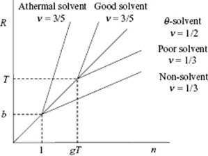
For athermal and good solvents (υ > 0) on a length scale r > ξ_T, the excluded volume repulsion is larger than kT. The polymer is then swollen with n/g_T thermal blobs and an end-to-end distance X ∼ ξ_T(n/g_T)^ν ∼ b(υ/b³)^2ν−1n^ν with ν = 3/5 (or ν = 0.588 using more sophisticated theory). For poor solvents (υ < 0) on a length scale r > ξ_T, the exclusive volume attraction is larger than kT. In this case, the blobs adhere to each other to form a dense globule. Assuming a dense packing of blobs, the size of this globule becomes R_glo ∼ ξ_T(n/g_T)^1/3 ∼ b²n^1/3/|υ|^1/3. The globule is approximately spherical and has a volume fraction , independent of the number of segments n. In Figure 13.5 the behavior for the various cases is sketched. Clearly, in reality the transitions indicated are less sharp than suggested by the graph in the figures.

Figure 13.5 Schematic of the relationship between the size R of a chain as a function of number of segments n where for each linear part R ∼ n^ν.

For poor solvents, the Flory theory requires some extension because for υ < 0 we find R = 0 as the optimum value. Two effects are relevant. The first is the effect of confinement in the blobs, while the second effect appears to be the excluded volume effect for two segments, to be extended even to three segments.

Consider first the confinement effect. The number of segments in a blob is given by g ∼ (R/b)². The energy cost per blob is kT, and because we have n/g blobs per chain that fully overlap we have the contribution F_con ∼ kTn/g ∼ kTnb²/R². Unfortunately, obtaining the optimum in the usual way, the result is still R = 0, and we therefore need to invoke other stabilization mechanisms in order to be able to describe the behavior of a polymer in a poor solvent.

For the excluded volume effect, we need the virial expansion of the interaction as expressed by Eq. (13.12), or actually its interaction part,

(13.28)

Recall that υ and ω represent the two-segment and three-segment contributions, respectively. The number density or concentration of segments inside a coil is given by c = n/R³. This implies that we have

(13.29)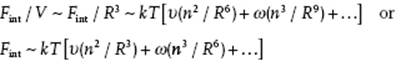

Adding this contribution to the terms that we already had, that is, kTυn²/R³ and kTR²/nb² from the original Flory treatment for good solvents and kTnb²/R² from the confinement contribution, we obtain

(13.30)

(13.31)

For the case that υ < 0 and ω > 0, the globule size R_glo becomes R_glo ∼ (ωn/|υ|)^1/3, so that for spherical segments with ω ∼ b⁶, we regain R_glo ∼ b²n^1/3/υ^1/3. For cylindrical segments ω ∼ b³d³ and the globule size becomes R_glo ∼ bdn^1/3/|υ|^1/3. The volume fraction in the globule is then . For the case of a non-solvent, υ ∼ −b²d, ϕ ∼ 1, and R_glo ∼ (bd²n)^1/3. Hence, the globule is fully collapsed, having a dense packing of segments, each of volume bd².

An approximate temperature dependence for υ can be obtained if we reconsider

(13.32)

and separate the integration in two parts. For r < b, βΦ(r) >> 1 and f = −1, while for r > b we have exp[−βΦ(r)] − 1 ≅ −βΦ(r) if βΦ(r) < 1. Hence, the integral becomes approximately

(13.33)

Defining now a characteristic temperature θ via

(13.34)

we obtain

(13.35)

This implies that the chain interaction parameter z becomes z ∼ υn^1/2/b³ ∼ (T − θ)n^1/2/T or z² ∼ υ²n/b⁶ ∼ n/g_T. Finally, we obtain for the number of segments in a thermal blob g_T ∼ b⁶/υ² ∼ n/z² ∼ [T/(T − θ)]². Hence, for T < θ we have R_F/R₀ ∼ R_F/n^1/2b ∼ b/υ^1/3n^1/6 ∼ z^−1/3 and the blob contracts. Oppositely for T > θ, R_F/R₀ ∼ R_F/n^1/2b ∼ z^2ν−1 ∼ z^2·(3/5)−1 ∼ z^0.2 and the blob swells. Overall, a fairly consistent description is obtained.