Liquid-State Physical Chemistry: Fundamentals, Modeling, and Applications (2013)

14.4. Diffusion Control

The main task in this section is to estimate the rate constants for diffusion k_D and k_−D. While the reactants may be either neutral or ionic, we start with ionic reactions.

The flux j_A – that is, the number of moles of ions crossing a unit area per unit time – of ions A with molarity c_A across a surface normal to the mass velocity v_A is given by

(14.32)

with the mobility u_A and electric field E. The factor z_A/|z_A| is introduced to fix the sign of the charge z_Ae of the ion A, since a positive ion has a positive flux in the direction of E. For this expression it is assumed that the flux is parallel to the electric field. With an additional concentration gradient, also assumed to be parallel to the electric field, the total flux in the direction of decreasing concentration becomes

(14.33)

with D_A the diffusion coefficient relative to the solvent. For the rate with which the reactant ions A and B approach each other we must replace D_A by D_A + D_B.

Consider now the first step of the scheme in Eq. (14.25), where the labels A and B represent ions with charge z_A and z_B, respectively. We assume that a gradient in c_B is present around each A ion, and vice versa. Using the Nernst–Einstein relation (Eq. 12.67)

(14.34)

and the relation between electric field E_z = −∂ϕ/∂z, with ϕ the electric potential, and potential energy Φ(r)

(14.35)

we obtain for the flux of B ions across a sphere of radius r around each ion A

(14.36)

where the overall negative sign disappears because the flux is now taken in the direction of increasing concentration. To illustrate the following argument more clearly, we ignore the dΦ_B(r)/dr contribution for the moment and add it again later.

The flow is J_B = 4πr²j_B, and we obtain for the molarity c_B(r)

(14.37)

The flow J_B can be taken outside the integral because under steady-state conditions the value of the flow is independent of the radius of the sphere. Because c_B(∞) represents the bulk molarity [B], the total result is

(14.38)

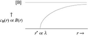
We now assume that, if ion A approaches ion B within a critical radius r*, a reaction occurs and c_B(r) = 0 for r < r* (Figure 14.3). This implies that the concentration gradient does not extend to r = 0 since all ions are lost reaching r*. The flow thus becomes

(14.39)

so that the rate of reaction reads

(14.40)

Figure 14.3 The behavior of c_B(r) and B(r) as a function of r.

The rate constant k_D is thus proportional to the diffusion constants, as expected, and a critical length r*.

Let us now introduce the dΦ_B(r)/dr contribution again. To solve the complete Eq. (14.36) we use a somewhat unexpected “Ansatz,” and note that if we differentiate the function

(14.41)

we obtain

(14.42)

From Eq. (14.36) we thus have

(14.43)

The integration corresponding to Eq. (14.37) becomes

(14.44)

where B(∞) is simply c_B(∞) = [B] and λ has the dimensions of length. Making the same assumption of a critical radius r* where c_B(r) = 0 and hence B(r) = 0, the total result is

(14.45)

(14.46)

Finally, we must link λ with r*, and this is done by assuming that the potential energy between two ions is given by

(14.47)

where the subscripts are omitted since the expression is symmetric in A and B. As usual, ε₀ and ε_r are the permittivity of vacuum and the relative permittivity, respectively. Substituting in Eq. (14.43) for λ and integrating results in

(14.48)

which, as it should, results in λ = r* for Φ(r) = 0 for r > r*. The behavior of the concentration profile c_B(r) and function B(r) as a function of r is sketched in Figure 14.3.

For the dimension of k_D we have to consider the dimension of D which is m² s⁻¹; hence, k_D will have dimension m³ s⁻¹. Conversion to molar quantities is achieved by multiplying with Avogadro's number N_A.

The rate constant for the reverse diffusion k_−D in the scheme of Eq. (14.25) is the reciprocal of the time in which A and B remain nearest neighbors. If specific interactions are absent, this quantity can be estimated from random walk diffusion d = (6Dt)^1/2, where d is the diffusion distance in time t. Hence, in this case k_−D is given by

(14.49)

Clearly, the controlling parameters for the controlled reactions are the charges z_A and z_B, the permittivity ε_r, and the diffusion coefficients D_A and D_B. Moreover, we need an estimate for r*, which is essentially an empirical parameter. We discuss the agreement with experiment after we have dealt with reaction control.