Liquid-State Physical Chemistry: Fundamentals, Modeling, and Applications (2013)
15. Some Special Topics: Surfaces of Liquids and Solutions
So far, in discussing the behavior of liquids and solutions we have limited ourselves to bulk fluids. However, in many cases interfaces are important, and in this chapter we deal with some aspects of these. In view of the wide range of phenomena associated with liquid interfaces, we limit ourselves to the thermodynamics and structure of planar (nonelectrified) surfaces of single-component liquids and binary solutions, the latter in relation to adsorption. For all other aspects, we refer to the literature.
15.1. Thermodynamics of Surfaces
To be able to discuss a multicomponent, multiphase system with interfaces, we need a concise notation. As before, we indicate the summation over the components, here labeled with the subscript i, by Σi. It is useful to refer to a particular component as the reference compound; this is usually taken to be the solvent and is labeled as 1. In considering two phases we have also to indicate the phase, and we do so by using a superscript (α) and (β) for the two bulk phases and (σ) for the interface, where the brackets are used to avoid confusion with exponentiation.
There are two approaches possible to describe the interfacial behavior of, say, a liquid and a vapor. First, the approach considering the interface as a real phase with volume, entropy, and so on (Figure 15.1a), as originated by van der Waals and Bakker and propagated in particular by Guggenheim. In this approach there are three phases to consider: the liquid; the vapor; and the interfacial phase (also called the interphase). For each phase the normal thermodynamic relations apply. There is only an additional work term for the interphase, to which we will come shortly. Second, we can associate the interface between two phases with a dividing (or geometric) plane, positioned in such a way that the total amount of a particular component, usually the solvent, is the same as if both bulk phases remained homogeneous up to that dividing plane (Figure 15.1a). This approach is due to Gibbs. Obviously, the dividing plane has volume zero but nevertheless it has other excess properties such as entropy and energy, which consequently can be positive or negative. The amount of component i in excess over the amount when both phases remain homogeneous up to the dividing plane as defined by component 1, is indicated by ![]() or per unit area as
or per unit area as ![]() , where A is the surface area. The quantity
, where A is the surface area. The quantity ![]() is addressed as surface excess. Obviously,
is addressed as surface excess. Obviously, ![]() . We will use both approaches.
. We will use both approaches.
Figure 15.1 (a) Schematic representation of the density profile over a liquid surface; (b) Schematic representation of the liquid–vapor interface, showing the difference in environment for a molecule at the surface and in the bulk.
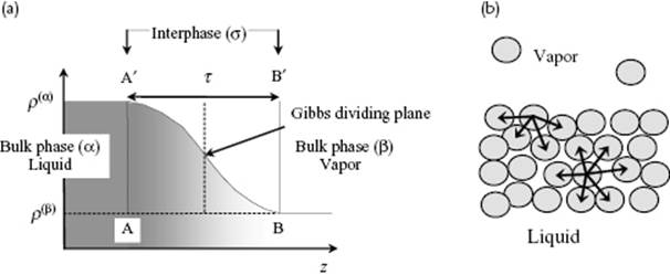
Simple considerations reveal that a surface must have an associated energy. If we consider the surface in comparison with the bulk, we note that there is a significant difference in surroundings of the molecules resulting in a lesser number of intermolecular interactions for the surface, even if the average structure in the surface (apart from the cut) remains the same as in the bulk. After surface creation, relaxation takes place resulting in an average structure in the surface different from the one in the bulk, but an excess energy remains (Figure 15.1b). Generally, the thickness τ of the interfacial region is extremely small, say, a few molecular diameters or about 1 nm for normal liquids and molecular solutions. A larger thickness might have to be considered if ions are involved in view of the associated Debye length (see Chapter 12).
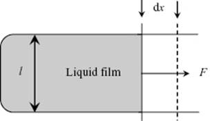
So far, we have treated liquids as homogeneous and obeying Euler's condition, so that total energy and entropy are additive if two volumes of liquid are added together. Moreover, we considered so far mainly volume work. However, surfaces have surface energy, so that if we create additional surface the work involved changes the various thermodynamic potentials, such as the Helmholtz energy. An elementary (though not so easy to carry out) experiment is the well-known surface extension experiment (Figure 15.2), which shows that to extend a surface by dA, an amount of work δW = γ dA is needed, where γ is called the interfacial tension1). Stability requires that γ > 0, consistent with the missing interactions in the molecular picture. This implies that, without other constraints present, for a liquid drop minimization of the surface (Gibbs or Helmholtz) energy leads to a spherical surface.
Figure 15.2 Schematic representation of a sliding-wire experiment to extend the area A of a liquid film at constant temperature T by dA = 2ldx, requiring a force F. Because the interface region of the film has a smaller density than the bulk of the film, during the process the volume changes and the process occurs actually at constant pressure P. Since the interfacial thickness τ is extremely small, say a few molecular diameters or about 1 nm, and therefore the interface volume V(σ) is small as compared to the bulk volume V(L), to a high degree of precision the process still occurs at constant volume V. In principle, the volume V could be kept really constant by carrying the experiment out in a closed set-up with cylinder and piston to keep the total volume constant. For a single-component liquid, because the work done is Fdx = γ dA, the surface tension γ represents both the surface stress per unit length and the Helmholtz (Gibbs) energy per unit area.
It is useful to consider the work γ dA somewhat more carefully. Consider to that purpose a system (Figure 15.1a), where the planes AA′ and BB′ are positioned in the bulk phases α and β parallel to the interface, so that their distance is τ and the volume of the interphase is V(σ) = Aτ. Recall that the pressure P = P(k) + P(c), with P(k) the kinetic and P(c) the configurational contribution (see Chapter 6), is the perpendicular force per unit area on an infinitesimal virtual test plane in the bulk phase, resulting from the collisions of all molecules on one side of this plane with all molecules at the other side. Consider now for a static liquid an infinitesimal cube with the xy plane parallel to the interface. The pressure on the yz-, xz-, and xy-planes is Pxx, Pyy and Pzz, respectively, and equilibrium of forces2) requires that ∂Pxx/∂x = ∂Pyy/∂y = ∂Pzz/∂z = 0. Because we have a planar interface, there is isotropy in the xy-plane, implying that Pxx = Pyy ≡ Pt with Pt the tangential pressure. This also means that Pxx, Pyy and Pzz are functions of z only. From ∂Pzz/∂z = 0, we have Pzz ≡ Pn with Pn the normal pressure, constant everywhere in the fluid. Actually, the bulk is fully isotropic and thus Pxx = Pyy = Pzz = P, where P is the hydrostatic pressure and thus Pn = P. For the interphase we have only planar isotropy so that Pt = Pt(z) varies with the height of the test plane within the interphase (Figure 15.3a). Summarizing so far, Pn = P everywhere and equal to Pt in the bulk phases, but Pt is possibly different from Pn in the interphase.
Figure 15.3 (a) The difference in attractive interactions between a test plane parallel and perpendicular to the interface. The hatched area represents the liquid, say phase (α), while the non-hatched area represents the vapor say phase, say phase (β). The range of interaction is indicated by the circles; (b) The contributions of the kinetic part of the pressure ![]() and the configurational part of the pressure
and the configurational part of the pressure ![]() and
and ![]() as function of z, that is, over the interphase (σ). While
as function of z, that is, over the interphase (σ). While ![]() for the two bulk phases,
for the two bulk phases, ![]() for the interphase. The integral over the difference Pn = P and Pt in the interphase represents the interfacial tension γ.
for the interphase. The integral over the difference Pn = P and Pt in the interphase represents the interfacial tension γ.
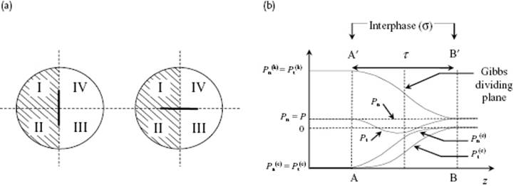
Experimentally indeed Pt ≠ Pn, as can be rationalized as follows. We recall that repulsive forces between molecules are much shorter ranged than attractive forces, so that we can neglect them and take the range of the attractive forces as finite. We take the test plane in the interphase (Figure 15.3), and note that the kinetic contribution to the pressure P(k) depends only on density (see Chapter 6). This is not true for the configurational part P(c). The decrease of attraction between molecules in quadrants I+II and III+IV for the orientation of the test plane parallel to the interface will be larger than the decrease in attraction between quadrants I+IV and II+III for the perpendicular orientation, because the density in both quadrants III and IV is small while quadrants I and II are densely populated [1]. The difference between P = Pn and Pt(z) integrated over the thickness τ of the interphase represents the interfacial tension
(15.1) 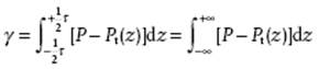
where the last step can be made because in the bulk phases P = Pt. Summarizing, the surface energy corresponds to the surface stress parallel to the surface.
Consider now a change in area dA, associated with a change in thickness dτ and a change in volume to V(σ) + dV(σ) for a constant amount of material. For the work in the direction perpendicular to the interface we have −PAdτ. The work in the direction parallel to the interface is −(Pτ−γ)dA, where the difference term, γ represents the interfacial tension. The total work done is then
(15.2) ![]()
and this expression replaces −PdV(α) as used for the bulk phase.
In the Guggenheim picture, the Helmholtz energy of the system F is defined by
(15.3) ![]()
where F(α), F(β) and F(σ) denote the Helmholtz energies of the two homogeneous phases and the interphase, respectively. A similar expression is used for U, V, S and ni. For the bulk phase we have
(15.4) ![]()
Clearly, the intensive properties T, P and μi do not require a phase superscript, since in equilibrium they are constant throughout the phases. Equation (15.4) is homogeneous of the first degree in the extensive properties V(α) and ![]() . Therefore, from Euler's theorem (see Appendix B) we have
. Therefore, from Euler's theorem (see Appendix B) we have
(15.5) ![]()
Similarly, for the surface phase we have
(15.6) ![]()
where γ is the surface tension. Equation (15.6) yields the Maxwell relation ![]() . Using Euler's theorem we find
. Using Euler's theorem we find
(15.7) ![]()
From Eq. (15.6) and (15.3) we easily obtain
(15.8) ![]()
For the Gibbs energy3) we use
(15.9) ![]()
so that
(15.10) ![]()
the last expression in correspondence with the same result for the bulk phase. Because F = F(α) + F(β) + F(σ) = −PV + Σiμini + γA, this requires that G = F + PV is taken as G = G(α) + G(β) + G(σ) + γA [deviating from the form of Eq. (15.3)]. Calculating dG we find
(15.11) ![]()
consistent with the sliding-wire experiment (Figure 15.2).
Differentiating Eq. (15.7) and subtracting the result from Eq. (15.6), we obtain
(15.12) ![]()
(15.13) ![]()
Equation (15.12) is the surface analog of the Gibbs–Duhem equation, known as the Gibbs adsorption equation. Approximating the activity ai in the expression for the chemical potential by the concentration ci, we have
(15.14) ![]()
This results in
(15.15) ![]()
It can be shown that this change is independent of the precise choice for the position of the planes [2] AA′ and BB′. Using the Gibbs approach with V(σ) = 0 is equivalent to taking the limit τ → 0 and referring the surface excess with respect to the resulting dividing plane determined by component 1. The result is
(15.16) ![]()
which is the form of the adsorption equation usually employed. Here, ![]() is the surface excess (or relative adsorption) of component i with respect to component 1. It can be shown that also this quantity is independent of the precise choice for the position of the dividing plane [3]. For a two-component system at constant T and P, we have
is the surface excess (or relative adsorption) of component i with respect to component 1. It can be shown that also this quantity is independent of the precise choice for the position of the dividing plane [3]. For a two-component system at constant T and P, we have ![]() . Evidently,
. Evidently, ![]() can be obtained by measuring the change in surface tension γ with concentration c.
can be obtained by measuring the change in surface tension γ with concentration c.
Let us focus for the moment on a single-component system, for example, the liquid–vapor system. In this case, Eq. (15.12) reduces to
(15.17) ![]()
Employing ![]() , where
, where ![]() indicates the molar entropy and
indicates the molar entropy and ![]() the molar volume, and eliminating dμ and dP, we obtain
the molar volume, and eliminating dμ and dP, we obtain
(15.18) ![]()
The last step can be made for surfaces between a liquid (α) and a vapor (β). In the interphase the density is comparable to that in the liquid so that ![]() , but
, but ![]() . Therefore, remote from the critical temperature,
. Therefore, remote from the critical temperature, ![]() . Similarly, employing
. Similarly, employing ![]() and g(σ) = Γμ = u(σ) − Ts(σ) + Pτ − γ with u(σ) = U(σ)/A and g(σ) = G(σ)/A, and eliminating
and g(σ) = Γμ = u(σ) − Ts(σ) + Pτ − γ with u(σ) = U(σ)/A and g(σ) = G(σ)/A, and eliminating ![]() ,
, ![]() and s(σ), the result is
and s(σ), the result is
(15.19) ![]()
where the last step can be made for the reason indicated before. For a created surface of unit area we may thus interpret γ as the work done, −T(∂γ/∂T) as the heat absorbed (the difference in entropy of surface and bulk for the same amount of matter, multiplied by T), and γ − T(∂γ/∂T) as the increase in internal energy (the difference in internal energy of surface and bulk for the same amount of matter).
If we use the Gibbs dividing surface for a single component system so that V(α) = 0, and position the dividing plane in such a way that ![]() , we obtain
, we obtain
(15.20) ![]()
and we see again that that the surface tension is equal to the surface Helmholtz energy per unit area4). For the (specific) surface internal energy one obtains
(15.21) ![]()
as expected, consistent with Eqs. (15.18) and (15.19).
Finally, as an aside, let us briefly consider the equilibrium of an infinitesimal, not necessarily planar, interfacial area with pressure P(α) on the one side and P(β) on the other side (at constant temperature and for constant amount of material). In the Gibbs approach, we have from Eq. (15.3), (15.4) and (15.6)
(15.22) ![]()
Since V = V(α) + V(β) is constant, we have dV(α) = −dV(β), resulting in
(15.23) ![]()
From differential geometry we learn that ![]() , where r1 and r2 are the radii of curvature in two orthogonal directions in the infinitesimal plane. It can be shown that
, where r1 and r2 are the radii of curvature in two orthogonal directions in the infinitesimal plane. It can be shown that ![]() , where R1 and R2 are respectively the minimum and maximum radii of curvature in two orthogonal directions, that is, the principal curvatures. Using
, where R1 and R2 are respectively the minimum and maximum radii of curvature in two orthogonal directions, that is, the principal curvatures. Using ![]() in Eq. (15.23), one usually refers to this as the Laplace equation, relating the surface tension to the pressure difference over a curved surface. It is here derived in an almost completely thermodynamic way. For a sphere, R1 = R2 = R and
in Eq. (15.23), one usually refers to this as the Laplace equation, relating the surface tension to the pressure difference over a curved surface. It is here derived in an almost completely thermodynamic way. For a sphere, R1 = R2 = R and
(15.24) ![]()
The above result can also be obtained using V = 4πR3/3 and A = 4πR2. It will be clear that for a planar surface R1 = R2 = ∞, resulting in P(α) − P(β) = 0.
Problem 15.1
Calculate the surface energy of water at 25 °C, given that the surface tension γ(0 °C) = 75.6 mJ m−2, γ(25 °C) = 72.0 mJ m−2, and γ(50 °C) = 67.9 mJ m−2.
Problem 15.2
Discuss the advantages and disadvantages of using either Eq. (15.17) or (15.20) as a basis for experimental work.
Problem 15.3
Show for a planar system containing bulk phases α and β and an interphase σ that the intensive quantities chemical potential μ, pressure P and temperature T are constant throughout the system.
Problem 15.4
Show for a planar system containing bulk phases α and β and an interface σ that the surface excess ![]() is independent of the position of the dividing plane. Hint: express
is independent of the position of the dividing plane. Hint: express ![]() in terms of ni,
in terms of ni, ![]() ,
, ![]() and
and ![]() , subtract
, subtract ![]() from the result, and note that one side is independent of the position of the dividing plane.
from the result, and note that one side is independent of the position of the dividing plane.