Liquid-State Physical Chemistry: Fundamentals, Modeling, and Applications (2013)

15.3. Gradient Theory

While the theory of fluids is somewhat complex, the theory for their surfaces is even more complex. We limit ourselves here to the classical picture initiated by van der Waals, often called (square) gradient theory, along the line as presented by Widom [28]. For more sophisticated treatments we refer to the literature, for example, Rowlinson and Widom [29], Davis [30], Safran [31], and Hansen and McDonald [32]. The basic idea of gradient theory is that, locally in the interphase, equilibrium prevails and therefore the total Helmholtz energy can be written as an integral over the local Helmholtz energy density, the latter being a function of density ρ only. We take the surface as the x–yplane and assume that the liquid is isotropic so that ρ is a well-defined function of z only, that is, ρ = ρ(z). For the interphase, the gradient in density is indicated by ρ′(z), where (here and in the sequel) the prime indicates the derivative with respect to the argument. The change in chemical potential μ of a liquid as a function of ρ is shown in Figure 15.5. In the interphase the density takes values between ρ_L and ρ_V which are excluded for the bulk phase by the equal-area rule. At any temperature in the two-phase region, the chemical potential in the interphase follows the metastable line f(ρ) between ρ_V and ρ_L, so that the “excess” Helmholtz energy F(ρ) is the difference between f(ρ) and the tie line indicated by μ₀. Hence, it reads

(15.41)

Figure 15.5 (a) Schematic representation of the change of chemical potential μ with density ρ for T < T_cri, T = T_cri and T > T_cri; (b) The excess Helmholtz energy F(ρ) between ρ_L and ρ_V.

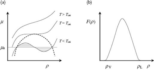
The lower limit can be taken as either ρ_V or ρ_L since, in view of the equal-area rule

(15.42)

with as consequence that F(ρ_V) = F(ρ_L) = 0. Figure 15.5 shows a schematic of F(ρ) indicating that, at any density between ρ_V and ρ_L, a positive excess energy is present.

The Helmholtz energy of the system would be minimized by an infinitely sharp transition between regions with density ρ_L and density ρ_V if a gradient in density in the interphase did not exist. However, a gradient ρ′(z) does exist and this gradient must stabilize the liquid at the densities in the interphase, since keeping the liquid at a density different from ρ_L and ρ_V will cost a significant amount of Helmholtz energy. In fact, the transition between ρ_L and ρ_Vcontributes to the excess Helmholtz energy, as can be seen in the following (this is in fact the same argument as used in Section 15.1). Consider two levels in the interphase with density ρ(z) and ρ(z + ξ), respectively. With r as the distance between a fixed point at level z and an arbitrary volume element dr at level z + ξ, we have an extra contribution to the Helmholtz (actually internal) energy density given approximately by

(15.43)

where ϕ(r) is the potential energy between molecules a distance r apart. The integration is over all space with r and ξ varying in the integration, while z and the point chosen at height z are fixed. The total excess Helmholtz energy is according to the above given by

(15.44)

The integral is function of a function, that is, a functional. The minimum of this functional of the density profile ρ(z), subject to the conditions ρ(−∞) = ρ_L and ρ(+∞) = ρ_V, provides the surface tension.

For small gradients we can expand ρ(z + ξ) in powers of ξ to second order and obtain

(15.45)

The first-order term does not contribute to the integral in Eq. (15.44), since the integration is over all space and ϕ(r) is a spherically symmetric function while ξ is odd. Using the same symmetry, the second-order term contributes one-third from what it would contribute if ξ² were to be replaced by r² (see also Justification 13.1). Therefore

(15.46)

The influence parameter m is proportional to the second moment of ϕ(r), and therefore measures the range of ϕ(r). A more elaborate analysis shows that m is related to the direct correlation function c(r). Approximating by c(r) ≅ c₀(r) − βϕ(r), with c₀(r) the correlation function of a reference system and β = 1/kT, results in

(15.47)

The last step can be made in view of the large weight given to ϕ(r) by the factor r². The term −½mρ (z)ρ′′(z) in Eq. (15.46) can be transformed by partial integration and, because the boundary terms vanish identically, this results in ½mρ′(z)². The final result is thus

(15.48)

Because the potential is attractive, we have ϕ(r) < 0, m > 0 and, consequently, γ > 0.

The minimum energy profile ρ(z) of Eq. (15.46) can be obtained by using the Euler condition (see Appendix B, Eq. B.61), which in this case becomes¹⁰⁾

(15.49)

Integrating, we obtain (note that F(ρ_L) = F(ρ_V) = 0):

(15.50)

from which we easily derive that

(15.51)

Using Eq. (15.48), the expression for the surface tension thus becomes

(15.52)

A second integration yields a parametric representation of the density profile

(15.53)

At liquid–gas coexistence, F(ρ) has two minima of equal depth. One is located at ρ = ρ_L and another at ρ = ρ_V. A simple parameterization, valid near the critical point, is

(15.54)

a temperature-dependent parameter. Substituting Eq. (15.54) in Eq. (15.53), we obtain

(15.55)

Here, λ = (m/2C)^1/2/(ρ_L − ρ_V) is a characteristic length for the interfacial width. Solving for ρ we find

(15.56)

For this profile the density ρ changes continuously from ρ_L to ρ_V, is anti-symmetric with respect to the mid-point z₀ as a consequence of the assumed form of Eq. (15.54), and diverges at the critical point. Within mean field theory (see Chapter 16) it appears that ρ_L − ρ_V ∼ (T_cri − T)^1/2 so that λ diverges as (T_cri − T)^−1/2.

Substituting Eq. (15.54) in Eq. (15.52), we find for γ close to T_cri

(15.57)

Hence, close to T_cri, γ ∼ (ρ_L − ρ_V)³ ∼ (T_cri − T)^3/2. Experiment and renormalization theory (see Chapter 16) show that the exponent really is about 1.26.

One of the better aspects of gradient theory is that, in principle, any equation of state can be used, whether experimental or theoretical. Moreover, although in principle derived for conditions near the critical point, it appears that its validity covers a much wider range [33]. Although rather successful qualitatively, for gradient theory a number of conceptual problems do exist. The density over the interphase is considered to be a well-defined function of the height in the interphase. Gravity is taken to localize the interface and to stabilize it against long-wavelength, thermally excited waves, the so-called capillary waves [34], which would smear out the profile even for, in principle, an infinitely sharp interface. For these aspects and other aspects we neglected, we refer to the literature.

Problem 15.9

Show that −½mρ(z)ρ′′(z) in Eq. (15.46) can be transformed by partial integration to ½mρ′(z)².

Problem 15.10

Verify Eq. (15.49).