Liquid-State Physical Chemistry: Fundamentals, Modeling, and Applications (2013)

2.3. Quantum Concepts

Although atomic and molecular phenomena require quantum mechanics for their description, for our discussion we need only some principles thereof and a few exactly soluble single-particle problems.

2.3.1 Basics of Quantum Mechanics

Since the discovery of quantum mechanics we know that in the Schrödinger representation the state of a system, that is, for the atoms or molecules at hand, is given by the wave function , where r stands for the full set of coordinates and t for time. This function and its gradient must be single-valued, finite, and continuous for all values of its arguments. A function satisfying these conditions is said to be well-behaved. It also must have a finite integral of its quadrate if integrated over the complete range of coordinates. Generally, we require that is normalized, that is,

where the asterisk denotes the complex conjugate. Schrödinger proposed that the time development of for a free particle with position¹⁵⁾ r and mass m is given by

(2.70)

where ħ = h/2π and h denotes Planck's constant. Using the de Broglie relation p = ħk with k = |k| = 2π/λ, where p is the momentum and k is the wave vector, we can write the wave function as exp(ik·r−ω t) with the circular frequency ω = 2πν, and, as usual, λ and ν representing the wavelength and frequency, respectively. Since the classical energy for a free particle is E = p²/2m, this suggests the operators

and these relations are accepted for all systems. In fact, every physical observable is represented by a linear Hermitian operator¹⁶⁾ acting on the wave function, for example, the position operator . The only possible values, which a measurement of the observable with operator can yield, are the eigenvalues a of the eigenvalue equation¹⁷⁾ with as the eigenfunction. For the coordinate operator the eigenvalues ξ of a single particle i are the values for which the equation

which is an ordinary algebraic equation, possesses solutions. Rewriting this as

it is evident that for this expression to be true either r = ξ or . This corresponds exactly to the definition of the Dirac δ-function (see Appendix B), which is thus the eigenfunction δ(r − ξ) associated with the operator for the eigenvalue ξ.

We note that the energy E for conservative systems is given by the Hamilton function in terms of the coordinates r and conjugated momenta p, that is, . We can therefore form the Hamilton operator (using a symmetrized function of r and p) leading to the time-dependent Schrödinger equation

(2.71)

For stationary solutions we may write

which, upon substitution in Eq. (2.71), leads to

As both sides are independent of each other, they both must be equal to a (so-called separation) constant, say E. Solving the time-dependent part leads to

while the space-part yields the time-independent Schrödinger equation

(2.72)

The latter is an eigenvalue equation that shows that the eigenvalue E represents the allowed quantum energy of the system. The constant C may be chosen to normalize Ψ(r), if necessary. In general a set of solutions is obtained where each solution characterized by a wave function Ψ_k(r) and associated energy E_k. The various wave functions Ψ_k(r) form, if normalized, a complete, orthonormal set, that is,

where the Dirac bra-ket notation¹⁸⁾ introduced. This is also true for the eigenfunctions of any operator, for example, the momentum operator −iħ∇. Here, we have

(2.73)

Normalization can be done in two ways. First, by periodic box normalization where we assume that the particle is contained in an arbitrary box of volume L³ and that the potential at x = y = z = 0 equals that x = y = z = L. We obtain, using ⟨Ψ_k|Ψ_l ⟩ = δ_kl = δ_kx,lxδ_ky,lyδ_kz,lz, C = L^−3/2. Second, by δ-function normalization where we employ a particular representation of the Dirac δ-function (see Appendix B), namely

The function sin(gx)/πx has a value of g/π at x = 0, oscillates with decreasing amplitude and period 2π/g with increasing |x| and is normalized, independent of the value of g. Hence,

Consequently, C = 2π^−3/2 using exp(ik·r) or C = h^−3/2 using exp(ip·r).

When a system is in an arbitrary state Φ the expected mean of a sequence of measurements of the observable with operator is given by

(2.74)

where is referred to as the expectation value and is to be interpreted as , where a_i denotes the measured value and ρ_i its probability of occurrence. If we expand Φ in terms of Ψ_k's, we have and the expectation value becomes

Hence, when the system is in a state Φ, a measurement of the observable A yields the value a_k with a probability , where c_k is the expansion coefficient (or probability amplitude) in the expansion of Φ in terms of Ψ_ks, or

(2.75)

The probability amplitude may be expressed in terms of Φ and Ψ_k as

(2.76)

If Φ is one of the eigenfunctions Ψ_l of , we obviously have ρ_k = ⟨Ψ_k |Ψ_l⟩ = δ_kl. In this case, the expectation value is thus equal to the eigenvalue a_l. The above considerations lead directly to the interpretation of the wave function. Consider the probability that a measurement of the position of a single particle i will give the value ξ. The eigenfunction corresponding to the coordinate operator r(i) for the eigenvalue ξ has shown to be Ψ_ξ = δ(r − ξ). From Eqs (2.75) and (2.76), we obtain

(2.77)

Hence, the probability of finding the particle i at r(i) = ξ is given by the square of its wave function evaluated at ξ. Generalization to many particles is straightforward.

An important next item is that conjugated variables, like the position coordinate r and momentum p or energy E and time t, cannot be determined precisely at the same time or, in other words, if one of the conjugated variables is exactly known, the other is fully undetermined. For the energy this is already clear: in a stationary state at any time t the energy is exactly E. In general any process that shortens the life time, broadens the energy level. Since transitions to other states are required for a change in time, there is a limited residence time Δt and this leads to a small uncertainty in energy ΔE given by ΔEΔt = ½ħ. More generally, if we define the variance by we have for any pair of conjugated variables a and b

(2.78)

which are known as the Heisenberg uncertainty relations. The implication for the pair coordinate r and momentum p is that a precisely localized particle has an indeterminate momentum, and vice versa.

Another important point is that particles also possess spin angular momentum, for which no classical analog is available, but which obeys the same quantization rules as orbital angular momentum. For an electron the eigenvalue for the spin operator is either ½ħ or −½ħ with the eigenfunctions generally denoted by α and β, respectively.

Finally, we focus our attention on systems with a Hamilton operator with additive properties. For many-particle systems the Hamilton operator is a function of the co-ordinates and the momenta of all the particles i,j, … , that is, . In a number of cases, however, the Hamilton operator is the sum (or can be approximated as the sum) of the operators for single particles i, that is, . These single-particle operators satisfy the (single particle) Schrödinger wave equation

(2.79)

where ϕ_k(i) and ε_k denote single-particle wave functions and eigenvalues (particle energies), respectively. The total wave function Ψ for the N-particle system can be taken as the product of the individual particle wave functions , so that the N-particle Schrödinger equation reads

(2.80)

and the total energy is given by . However, we note that the individual particles in a system are indistinguishable. This implies that the wave function must be either symmetrical or anti-symmetrical with respect to exchange of particle coordinates, including spin. Electrons are particles with a half-integer spin, the so-called fermions (or Fermi–Dirac particles), for which the wave function must be anti-symmetric in the coordinates of all electrons. A direct consequence, usually referred to as Pauli's principle, is that each system state can be occupied with only one electron. For an electron with spin ½ this implies either spin up (½ħ) or with spin down (−½ħ). Making allowance for Pauli's principle, a many-electron wave function can be expanded in anti-symmetrized products of one-electron wave functions (or spin orbitals) ϕ_j, each ϕ_j consisting of a spatial part (or orbital) and a spin function (σ_j = α or β). For this the permutation operator is used, which permutes the coordinates r of the wave function. A permutation is either odd or even, dependent on the number of binary switches in coordinates that is required to realize that permutation. A completely anti-symmetrized wave function Ψ^(A) is obtained by combining all N! permutations of the wave function Ψ = Ψ(r₁, r₂, … ,r_N), that is, by taking

(2.81)

So we have or 1 for an odd or even permutation, respectively. For future reference we include the prefactor in the operator by writing . A convenient form for such an anti-symmetrized product is the Slater determinant, in shorthand written as

(2.82)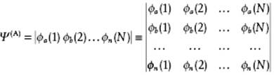

where (i) denotes the coordinates of an electron including spin and N the number of electrons. Similarly, for integer spin particles, the so-called bosons (or Bose–Einstein particles), the wave function must be symmetric in all the coordinates of the particles and the system states may contain any number of particles. This symmetry can be realized by taking the permanent of individual particle wave functions indicated by

(2.83)

The permanent is constructed similarly as the determinant but upon expanding one takes all signs as positive. Hence, always. In order to obtain a normalized wave function Ψ, if all ϕ's are orthonormal, one has to include a normalization factor C = [N!Π_i(n_i!)]^−1/2

for fermions and bosons, respectively. Note that for Fermi–Dirac particles C becomes C = (N!)^−1/2 because all n_i are either 1 or 0. The factor C is often incorporated in the definition of the (anti-)symmetrized product function so that we write for the wave function Ψ = |ϕ_a(1) ϕ_b(2) … ϕ_n(N)| or even, assuming a fixed order of coordinates Ψ = |ϕ_a ϕ_b … ϕ_n|. The same convention is used for the symmetrized product function. A straightforward calculation shows that for the Hamilton operator with additive properties the N-particle system eigenvalue is still

When , the energy E is no longer the sum of the particle energies and the product function and determinant (or permanent) no longer yield the same energy.

To conclude this section we mention that the number of exact solutions for realistic systems is very limited in quantum mechanics¹⁹⁾. Therefore, as has been emphasized many times before, the Schrödinger equation needs drastic approximations in almost all cases, even to obtain approximate solutions. We indicate here only the solutions of a few, exactly solvable single-particle problems, namely the particle-in-a-box, the harmonic oscillator, and the rigid rotator. Thereafter, we briefly discuss some approximation methods. For our discussion of liquids and solutions, the basic concepts and examples discussed will more than suffice. In fact, the existence of energy levels is the most important aspect for the basis of statistical thermodynamics.

Problem 2.16

Show that the eigenvalues of a Hermitian operator are real.

Problem 2.17

Prove the orthogonality of the eigenfunctions of a Hermitian operator.

Problem 2.18

Show that the squared deviation of the energy from its expectation value for a stationary state is zero, that is, .

Problem 2.19

Write explicitly the expression for two-electron determinant wave function. Show that this expression can be separated in a spatial and a spin factor.

Problem 2.20*

Verify that the total energy for an operator for a determinant wave function.

Problem 2.21*

Calculate the energy for a two-electron product and determinant wave function using the Hamilton operator . Show that the total energy is no longer the sum of the single particle energies for the determinant.

2.3.2 The Particle-in-a-Box

For a particle in a one-dimensional box the potential energy is given by

(2.84)

The kinetic energy operator is

(2.85)

where m is the mass of the particle, so that the Schrödinger equation reads

(2.86)

The solutions are

(2.87)

where n = 1,2, … is a positive integer, the so-called quantum number, arising since only for discrete wavelengths the solution obeys the boundary conditions. These wavelengths are given by λ = 2w/1, 2w/2, … , 2w/n with allowed energies

(2.88)

where k is the wave vector and p the momentum. In the ground state with n = 1, the energy is still not zero and the wave function represents a standing wave. For a three-dimensional box with potential energy Φ(r) = 0 for 0 < r < wand Φ(r) = ∞; otherwise, the energy levels are

(2.89)

If one of the dimensions of the box is equal to another, the energy levels become degenerate, that is, there are two (or more) states with the same energy. For example, if w₁ = w₂ = w₃ the energies for states n = (1,2,2), n = (2,1,2) and n = (2,2,1) are the same, and the system is said to be three-fold degenerate. Using periodic boundary conditions Φ(0) = Φ(w) = constant, instead of the fixed box boundary conditions given by Eq. (2.84), a similar procedure will lead to the same expression for E_n but with the factor 8 replaced by 2. In this case, n = (n₁,n₂,n₃) ∈ (±1,±2, …) and the wave functions exp(ip·r/ħ) = exp(ik·r) represent running waves.

2.3.3 The Harmonic Oscillator

For a one-dimensional harmonic oscillator the potential energy with force constant a and the kinetic energy operator are given by

(2.90)

respectively, so that the Schrödinger equation reads

(2.91)

The solutions for the wave functions are

(2.92)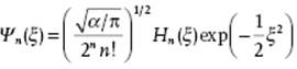

and where H_n(x) are known as Hermite functions defined by

Explicitly the first few Hermite functions are

The energy levels are given by

(2.93)

For a three-dimensional oscillator with potential energy (shifting the origin with x₀, y₀ and z₀)

(2.94)

the energy levels are given by

(2.95)

Again, if one of the frequencies is equal to another, the system is degenerate. For example, if ω_x = ω_y = ω_z, for states n = (1,1,2), n = (1,2,1) and n = (2,1,1) the energy levels are the same and given by

and the system is three-fold degenerate. Finally, we note that the presence of the zero-point energy ½ħω for the ground state n = 0 is in accord with the uncertainty relations. If the oscillator had no zero-point energy, it would have zero momentum and be located exactly at the minimum of Φ(r). The necessary uncertainties in position and momentum thus give rise to the zero-point energy. Finally, for completeness, we mention that the selection rule for transitions between levels is given by Δn = ±1.

2.3.4 The Rigid Rotator

For the rigid two-particle (atom) rotator there is no potential in the conventional sense, but there is the constraint that the distance between the two particles of the rotator should remain constant. Hence, the Schrödinger equation reads

(2.96)

where μ indicates the reduced mass of the rotator given by 1/μ = 1/m₁ + 1/m₂, m₁ and m₂ are the masses of the two particles. The constraint is taken into account as follows. Rigid rotation is realized if we suppose that the two rigidly connected particles rotate freely over a sphere. For this problem it is convenient to think in terms of polar coordinates, where the radial variable or radius r is fixed but the angular coordinates θ and φ are free. The Laplace operator ∇², expressed in polar coordinates and acting on a scalar x, is expressed by

(2.97)

The Legendre operator Λ² is the angular part of the Laplace operator. The constraint r = constant implies that the radial part of the Laplace operator can be skipped. Hence, the Schrödinger equation becomes

(2.98)

where I = μr² is the moment of inertia. The solutions for this equation are the spherical harmonics, conventionally indicated by Y_lm(θ,φ), and characterized by the two quantum numbers [9] l and m. The number l = 0,1,2, … indicates the overall angular momentum, given by [l(l + 1)]^1/2ħ, while the number m = −l,−l + 1, … ,l − 1,l indicates the angular momentum in a specified direction, often taken as x, and given by mħ. The energy expression is independent of the quantum number m and becomes

(2.99)

The above notation is the conventional one in quantum mechanics for the solution of the angular part of the Laplace operator. However, in spectroscopy the symbol for the quantum number l is usually replaced by J, and we will also do so. Each energy level is thus characterized by the quantum number J corresponding to 2J + 1 quantum states, that is, the degeneracy is 2J + 1. Again for completeness, we mention that the selection rule for transitions between levels is ΔJ = ±1.