Liquid-State Physical Chemistry: Fundamentals, Modeling, and Applications (2013)

15.5. Statistics of Adsorption

Apart from a thermodynamic description of liquid surfaces, another route is to use a statistical mechanical approach. We do so briefly in this section, limiting ourselves again to surfaces, and to that purpose consider a binary system for which we denote the bulk composition with A_1−xB_x and the surface composition A_1−yB_y. We again use a lattice-type model, and assume that only the first molecular layer has a composition different from the bulk. As before, the components are indicated by subscript i, while the surface and bulk phase are indicated by superscripts (σ) and (α), respectively. We start with an ideal solution and thereafter consider the influence of nonideality.

We recall that the chemical potential of component i is given by

(15.70)

where and are the standard chemical potentials of the pure components in the bulk and the surface, respectively, while x and y denote the mole fractions. Further, at equilibrium we have . From these equations we easily obtain

(15.71)

The Helmholtz energies are then given by

(15.72)

For a one-component system the surface tension is given by , so that

(15.73)

where a_i = A/N_i denotes the area per molecule. If we subtract Eq. (15.71-2) from Eq. (15.71-1) and Eq. (15.72-2) from Eq. (15.72-1) and insert Eq. (15.73) for both components, we obtain

(15.74)

This is the adsorption equation for ideal solutions.

We now introduce interactions and “change gear” to statistics, employing the grand (canonical) partition function Ξ in connection with the lattice model. Note that Ξ is the proper partition function to use, since we keep μ_i, N and Vconstant (see Chapter 5). The configurational partition function of the surface layer Q^(σ) is given by

(15.75)

where

(15.76)

The energy U^(σ) is evaluated as for a regular solution (in the zeroth approximation) and reads, using as before the interaction energy 2w = 2w_AB − w_AA − w_BB,

(15.77)

Here, is the coordination number for “bonds” in the surface layer with composition A_1−yB_y, and is the coordination number for “bonds” between the surface layer and the first bulk layer, so that the total surface coordination number reads (e.g., for a FCC (111) plane and ). The grand partition function becomes

(15.78)

We now use the maximum-term method (see Justification 5.4), replacing the sum by its largest term and obtain

(15.79)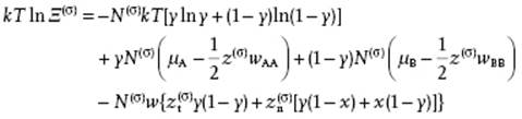

The equilibrium condition is

(15.80)

and leads to

(15.81)

From and Eq. (15.71) we obtain

(15.82)

so that combining Eq. (15.81) and (15.82) gives

(15.83)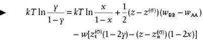

This is the equivalent of Eq. (15.74) in the zeroth approximation. We see that the surface tension term −(a_Bγ_B − a_Aγ_A) is replaced by ½(z − z^(σ))(w_BB − w_AA), while the interaction term with w is obviously absent for the ideal solution.

Estimating w_ii from the heat of vaporization L_i in the nearest-neighbor approximation L_i = −½zN_Aw_ii (with N_A = Avogadro's constant) and w from the heat of solution L_AB of component A in component B (or vice versa from L_BA), we have

(15.84)

Note that the heat of vaporization is counted positive, while the bond energy is counted negative. In the zeroth approximation of the regular solution theory ΔL_AB = ΔL_BA. Experimentally, this condition is only exceptionally fulfilled, which indicates a need for further improvement. However, the approach does provide a clear basis for a picture in which the surface tension – that is, the surface Helmholtz energy – is estimated as, with again N_A as Avogadro's number,

(15.85)

Using this approximation we obviously neglect entropy terms and have identified ½zw_ii with and ½z^(σ)w_ii with . The discussion in Section 15.2 showed that, numerically, the difference is far from negligible. The fraction of missing “bonds” (z−z^(σ))/z, as also indicated in Section 15.2, is ∼1/4.