Liquid-State Physical Chemistry: Fundamentals, Modeling, and Applications (2013)

15.6. Characteristic Adsorption Behavior

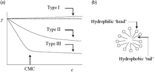
Generally, three types of behavior of γ for the various types of solutes with concentration can be distinguished, as illustrated schematically in Figure 15.6. Type I behavior includes hydrophilic compounds which prefer to be in water and therefore deplete at the interface, resulting in a, generally small, increase in γ. The most common examples are salts such as NaCl. As an illustration we quote that, at room temperature, γ rises from ∼72.6 mJ m⁻² for pure water to ∼76.0 mJ m⁻² for a 2 M aqueous solution of NaCl. Type II behavior comprises the hydrophobic compounds; these do not prefer to be in the water and therefore segregate at the interface, resulting in a decrease in γ. Aliphatic alcohols with a somewhat longer chain such as hexanol provide an example. Type III behavior includes amphiphilic compounds or surfactants that generally contain strongly hydrophobic “tails” and strongly hydrophilic “heads.” One can distinguish between anionic surfactants generating negative molecules (and a positive counterion) and cationic surfactants generating positive molecules (and a negative counterion). Typical examples are sodium dodecylsulfate (SDS; C₁₂H₂₅OSO₃Na) and hexadecyl trimethylammonium bromide (CTAB; C₁₂H₂₅N(CH₃)₃Br). Moreover, one has nonionic surfactants containing highly polar groups, such as polyethylene oxide, and amphotericsurfactants carrying a positive and negative charge while being on the whole neutral. The cationic and anionic compounds strongly enrich at the interface because their tails prefer to be out of the water while their heads prefer to be in the water. The polar groups of the nonionic surfactants prefer the water phase with a similar effect. Most surfactants are anionic, followed by nonionic surfactants. Cationic surfactants often pose environmental problems, while amphoteric surfactants are generally expensive and therefore are only used for special applications. Surfactants generally enrich strongly at the interface, so that γ is decreased considerably at small concentrations. Above a certain concentration they do not further enrich at the surface (the surface is “occupied”) but rather form micelles, clusters of typically 50 surfactant molecules in which the tails stick together in order to minimize the contact with water, and of which the structure is shown schematically in Figure 15.6. This concentration is called the critical micelle concentration (CMC). The solubility of surfactants is generally low but increases with temperature. The temperature at which the CMC equals the solubility is normally addressed as the Kraft temperature. Above this temperature, micelle formation is possible and surfactants are much more active above this temperature than below.

Figure 15.6 (a) Schematic representation of the interfacial tension with concentration for hydrophilic (type I), hydrophobic (type II), and amphiphilic solutes (type III, surfactants). The CMC is indicated; (b) Schematic representation of the structure of micelles occurring at c > c_CMC for surfactants, where the hydrophilic head is indicated by O and the hydrophobic tail by –––.

15.6.1 Amphiphilic Solutes

For amphiphilic solutes (surfactants), we may suppose that the concentration in the bulk is small and that segregation occurs essentially at the first surface layer (a higher concentration leads to micelles). Thermodynamically, this means that we assume that , so that and . We discuss a kinetic and a statistical–mechanical approach, both leading to the Langmuir isotherm.

For the kinetic approach we consider the surface as a plane with a certain density of surface sites. The process in the surface layer can be represented as a chemical reaction where the solute dissolved in the bulk (B) “reacts” with an empty surface site (S) to an occupied adsorbed site (A); that is, B + S ↔ A. Obviously, we assume that the molecules at the surface do not interact. Since the solubility is low, we approximate the activity a by concentration¹¹⁾c = N_B/V, where N_B is the number of dissolved molecules in the volume V. We denote the fraction occupied surface sites by θ, that is, θ = N_A/N_max, where N_max is the number of sites at monolayer coverage. Hence, N_S/N_max = 1 − θ. The equilibrium constant K for this adsorption “reaction” is then

(15.86)

usually called the Langmuir adsorption isotherm. The amount of segregated material Γ^(σ) is then, with Γ_max a proportionality constant representing monolayer coverage,

(15.87)

The latter form can be used for regression analysis of experimental data.

Before we discuss the behavior and some consequences of the Langmuir isotherm, we first derive it via statistical mechanics. In this approach, we consider the solvent and the surface phase and equate the chemical potential of the solute in the bulk phase μ^(α) with that of the surface phase μ^(σ). In view of the limited solubility, we assume ideal behavior so that the N solute molecules can move freely through the solvent with volume V with potential energy ϕ_α. Hence, we have for the partition function z^(α) of a single molecule (see Chapter 5)

(15.88)

where is the internal partition function and the external partition function, representing the translation motion of the molecule as a whole, with Λ ≡ (h²/2πmkT)^1/2 the thermal length. For the total partition function Z^(α)and Helmholtz energy F^(α) in the bulk we have, respectively,

(15.89)

so that

(15.90)

For the surface we suppose that we have M sites of which S are occupied. Hence, the fraction adsorbed molecules θ = S/M and the fraction of nonoccupied sites is 1 − θ = (M − S)/M. The partition function for a single molecule becomes

(15.91)

where similar labels are used as for the bulk. The total partition function Z^(σ) and Helmholtz energy F^(σ) for the surface then read, respectively,

(15.92)

where the factor M!/S!(M − S)! is introduced in view of the indistinguish­ability. Employing the Stirling approximation for the factorials, we have . The chemical potential μ^(σ) accord­ingly becomes

(15.93)

Equating μ^(α) with μ^(σ) we obtain, using for the bulk concentration c = N/V,

(15.94)

equivalent to Eq. (15.86) if we take¹²⁾ K = b(T).

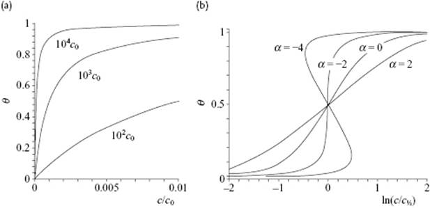
Let us now evaluate the Langmuir behavior. For small c, the increase in θ ≅ Kc, that is, the occupied surface site fraction is linear in c, while for large c, we have θ → 1, that is, the occupied surface site fraction saturates at 1. This behavior is displayed in Figure 15.7 for various values of K. Taking K = 10⁴c₀ as an example, we note that θ ≅ 1 at c/c₀ ≅ 0.002, so that the CMC in this model will be about 0.002c₀. A few more remarks can be made. First, recall that the equilibrium constant for adsorption K is related to the Gibbs energy of adsorption G_ads by K = exp(−G_ads/kT), to be compared with Eq. (15.94). Having determined K as a function of T, all other thermodynamic properties, such as the heat of adsorption, can be determined in the usual way. Second, substituting the Langmuir isotherm Γ^(σ) = Γ_maxθ = Γ_maxKc/(1 + Kc) in the Gibbs adsorption expression Γ^(σ) = −(RT)⁻¹∂γ/∂ lnc and solving for γ, one obtains the Szyszkowski equation [35] reading

(15.95)

which appears to describe experimentally the amount of adsorbed material often rather well.

Figure 15.7 (a) The Langmuir isotherm θ(c) = K(c/c₀)/[1 + K(c/c₀)] for K = 10²c₀, 10³c₀, and 10⁴c₀; (b) The Fowler–Guggenheim adsorption isotherm for various values of α = zw/kT. The critical value is α = −2, while α = 0 corresponds to the Langmuir isotherm.

Obviously, other assumptions lead to different adsorption isotherms. In fact, if we assume that the molecules at the surface do attract each other so that the energy changes by 2zwθ, where z denotes the surface coordination number and 2w the energy when a new pair of neighbors is formed, but that the surface entropy is not affected¹³⁾, we have

(15.96)

This leads to the Fowler–Guggenheim adsorption isotherm reading

(15.97)

Plotting θ as a function of ln(c/c_½), where c_½ is the concentration where θ = ½, we see that this isotherm produces a van der Waals shape with two loops for α = zw/kT < −2, characteristic of a phase transformation. The critical temperature is thus determined by , occurring at θ_cri = ½. Figure 15.7 shows the behavior for the various values of α. In view of the fact that the solution is obtained via the zeroth approximation, more sophisticated solutions lead to different values for . For example, the first-order approximation leads for a square lattice (z = 4) to while an exact solution yields (see Appendix 3).

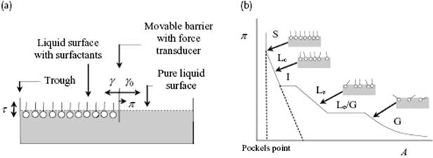
Another extreme for a liquid surface would be that the adsorbed molecules can move freely, much like a 2D-gas. This is suggested by the fact that the surface pressure π = γ₀ − γ, where γ₀ is the surface tension of the pure liquid and γ is the surface tension of the solution, for low concentration c is linearly related to c, that is, π = λc, with λ a constant. The surface pressure is usually measured with a surface pressure balance, often denoted as Langmuir–Blodgett trough, of which a schematic is shown in Figure 15.8. On one side of a movable barrier, surfactant is added to the surface while the other side has a pure water surface. By measuring the surface pressure as function of surface area A and using the Gibbs adsorption expression −dγ = dπ = kTΓ dlnc with in conjunction with the experimental relation π = λc, we obtain

(15.98)

Figure 15.8 (a) Schematic representation of a Langmuir–Blodgett trough; (b) Schematic representation of the surface pressure π = γ₀ − γ versus surface area A and the associated structure, showing the regimes of gas-like (G), liquid-expanded (L_e), liquid-condensed (L_c), and solid (S).

This expression resembles that of the ideal gas law, and suggests similar improvements for the surface as has been used for bulk gases. By employing the van der Waals approximation, in analogy with the 3D expression (P + aρ²)(1 − bρ) = ρRT (see Chapter 4), for 2D reading

(15.99)

with a and b parameters and where θ (or σ = 1/θ) in 2D corresponds to ρ (or V_m = 1/ρ) in 3D, the van der Waals adsorption isotherm becomes, with the constant ε = 2a/b,

(15.100)

This isotherm predicts a phase change, similarly as in the case of localized adsorption with attractive interaction. Characteristics are θ_cri = ⅓ and . This isotherm is not symmetric around θ = ½. While for θ > ½, the vdW isotherm resembles the Langmuir isotherm, for θ < ½ it decreases much more rapidly and resembles the Fowler–Guggenheim isotherm.

In fact, the surface pressure π = γ₀ − γ of a film of amphiphilic molecules as a function of area A shows several features akin to gas compression. A schematic is provided in Figure 15.8, which shows the regimes labeled solid (S), liquid-condensed (L_c), intermediate (I), liquid-expanded (L_e), and gas (G). The structure changes during compression and this change is also schematically indicated. We have already mentioned the gas-like region in which the tails still make a considerable amount of contact with the liquid surface. In the liquid-expanded region the surface contains still a disordered, homogeneous distribution of molecules, but the tails lift off the surface. There is an intermediate region where gas-like and liquid-like areas coexist. The liquid-condensed phase is actually more solid-like because the tails are already aligned. Here, the molecules are relatively (surface) close-packed but are still rather mobile. In the solid-like region, the molecules are really close-packed and compressed to each other. Occasionally, a phase intermediate between the L_c and L_e phase is observed. The transition point between the S and L_cphase, the Pockels point, is a measure for the area occupied by the molecules. By knowing the amount of molecules on the surface, one can estimate the molecular area, since at that point they are just close-packed.

A pioneering experiment was that of Langmuir [36], who studied amphiphilic molecules with different chain lengths. For example, he used CH₃(CH₂)_nCOOH with n = 14, 16 and 24, which resulted in 21, 22 and 25 Ų, respectively. From this, Langmuir concluded that the “head” area or COOH area is about 23 Ų, independent of the chain length. This field has undergone tremendous development since then and now contains many interesting structures and phenomena, detailed discussions of which are available elsewhere [37, 38].

It should be noted that, although the interpretation of the above transition between solid and liquid compressed phase of the adsorption isotherm is straightforward, and has generally been accepted as correct, debate still persists in the literature [39]¹⁴⁾

.

15.6.2 Hydrophobic Solutes

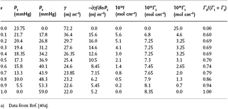
Although, for hydrophobic solutes the change in γ is relatively small, even with fully soluble solutes segregation and orientation still occur. To illustrate such behavior we use the example of water and ethanol. Estimating the surface energy of hydroxyl groups by extrapolation from water as ∼190 mJ m⁻², and that of hydrocarbon groups as ∼50 mJ m⁻², one can easily reach the conclusion that the hydrocarbon tails should “stick out” of the solution. Supporting this suggestion is the fact that the actual surface tension of ethanol is 22 mJ m⁻², which is quite similar to the value for hydrocarbons. To illustrate such behavior further, we can use the data on water–ethanol solutions [40]. From measurements of the vapor pressure of water P₁, of ethanol P₂, and the surface tension γ, the quantity −∂γ/∂ln P₂ can be calculated, and thus . Table 15.4 provides the relevant data. A useful intermediate is . Estimates for the individual values of Γ₁ and Γ₂ can be made only if extra assumptions are made. If we assume that the surface is covered with a monolayer, and that each molecule contributes a constant area A_i to the interface, we have A₁Γ₁ + A₂Γ₂ = 1. Estimating the molecular areas for H₂O and CH₃CH₂OH as A₁ = 0.4 × 10¹⁰ cm² mol⁻¹ (A₁/N_A ≅ 7 Ų) and A₂ = 1.2 × 10¹⁰ cm² mol⁻¹ (A₂/N_A ≅ 20 Ų), one can estimate Γ₁ and Γ₂ from the above two equations, as given in Table 15.4. Further calculating y = Γ₂/(Γ₁ + Γ₂), which can be considered as the mole fraction in the surface, we see that y increases rapidly with the bulk mole fraction xand reaches already y ≅ 0.6 at x = 0.1. Later analysis supports this image, including the sticking out of the surface of the hydrocarbon tail [41] (suggesting an average angle of ∼40 ° with respect to the surface with a distribution width of about 30 °). Even for this relatively simple system the structure of the surface layer appears to be not completely known.

Table 15.4 Mixture of water and ethanol at 25 °C.^a)

The molecular structure of liquid solution surfaces is still intensively investigated. Today, the literature is extended and many – often opposing – views have been expressed. Important experimental methods, sum-frequency spectroscopy [42] and neutron reflection [43], as well as theoretical methods [44], have been reviewed.

15.6.3 Hydrophilic Solutes

Contrary to hydrophobic and amphiphilic solutes, hydrophilic solutes show depletion at the interface, leading to an increase in surface tension, albeit of a much smaller magnitude as compared to the decrease in surface tension for the other two types of solute. Theories fall into three groups: (i) direct calculation of the work of separation for a surface originally in the interior of the solution; (ii) calculation of the depletion, followed by the use of the Gibbs adsorption equation; and (iii) calculation by statistical mechanics using the pair correlation function using an extended Kirkwood–Buff approach. Here, we briefly limit the discussion to theories of the second type, since those of the first type are used only to a limited degree, while those of the third type are limited to more or less spherical molecules.

Within the theories of type two, two basic pictures have been used. In the oldest case, the increase in γ has been modeled by Wagner, Onsager, and Samaras [45], invoking the image charges that repel the ions from the surface. In this picture, polarizability is entirely neglected, but Stairs [46] has modified the model so as to include this effect. The second picture uses the fact that the hydration shell of ions cannot stick out of the surface. Disruption of the hydration shell would involve a large amount of energy as the hydration energies are large; hence, to keep the shell intact ions cannot approach the surface too closely [47]. Again, the field is wide, but has been reviewed [48].

It should be mentioned that an alternative picture for the surface structure of salt solutions has been proposed [49] on the basis of MD simulation in which the polarizability of the ions plays a significant role. Whilst for the small and hardly polarizable ions, such as Na⁺ and F⁻, depletion does indeed occur, for the larger and more polarizable ions an enrichment was actually calculated. This was attributed to an anisotropic solvation, leading to a substantial dipole on the ion. The positive ions were indeed depleted from the surface, whereas the negative ions were enriched. The solvated-ion-dipole/water-dipole interactions were shown to compensate for the loss of pure-ion-charge/water-dipole interactions. This picture was consistent with, for example, surface potential measurements.

Problem 15.11: Langmuir isotherm

Show that, taking θ = n/n_max = Kc/(1 + Kc), with n the number of moles adsorbed and n_max the number of moles adsorbed at full monolayer coverage, the Langmuir isotherm can also be linearized as c/n = (1/n_maxK) + (c/n_max).

Problem 15.12

Derive Eq. (15.95).

Problem 15.13: van der Waals isotherm

Using the 2D vdW equation (π + aσ⁻²)(σ − b) = kT and the Gibbs adsorption expression Γ = −(RT)⁻¹∂γ/∂ lnc, derive the vdW adsorption expression Eq. (15.100). Hint: write d lnc as a function of dπ and integrate the resulting expression term by term.