Microreactors in Organic Chemistry and Catalysis, Second Edition (2013)

4.4. Automated Multi-Trajectory Optimization

In more complex reaction schemes, the terrain of the objective function will not point so directly to the optimal conditions. Thus, an expanded multi-trajectory optimization system is designed, allowing for the optimization of such a complex reaction system. This analysis takes into account the changing behavior of the objective function by re-analyzing the objective terrain and changing the search direction during the optimization [39, 40].

This method focused on the overall approach used to conduct reaction optimizations, regardless of the reaction or the actual objective function. Thus, it would be possible to interchange objectives or even reactions using the same methodology. A well-known method that is often used to accomplish this is DoE, but this approach assumes that the objective function can be well modeled over its entirety by a low-order function. Here, no such assumption is necessary, and this approach is intended to be extendable to more complex systems where design of experiments would fail to adequately capture the nature of the objective function.

Most previous studies have monitored performance only intermittently and at a single wavelength. In this example, the reaction progression was analyzed quantitatively via in-line ATR–FTIR using Mettler Toledo's ReactIR micro flow cell, which has a 51 μL flow cell equipped with a multi-pass diamond window to allow for continuous monitoring of the mid-IR range [41]. This analytical technique has previously been used in characterizing system dispersion and chromatographic effects, reaction screening, and monitoring reactor failures, though none of the data were used to quantitatively assess reaction progress, much less investigate reaction kinetics [42, 43]. Additionally, use of in-line IR measurements in process optimization has typically been done by testing a few settings of process variables, changing one at a time, and observing the relative size of the desired peak, without quantitative analysis or investigation of parameter interactions [44].

The IR micro flow cell enables monitoring of the reaction's approach to steady state, ensuring that steady-state data are used for analysis. Thus, the next set of reaction conditions can begin as soon as the previous steady state had been reached and assessed, rather than waiting a fixed number of residence times and assuming that steady state has occurred, as done previously [35, 38]. Moreover, this analysis can be performed directly in-line at reaction concentrations by using the entire reactor effluent, rather than requiring significant dilution of only a small reaction sample, as with HPLC sampling, enabling better characterization of system fluctuations and non-destructive analysis between unit operations. It would also be possible to monitor the reaction with in-line IR in the presence of unknown reaction species (intermediates or byproducts); however, as with any measurement technique, each reaction species would have to be isolated and calibrated to be certain of quantitative analysis. In addition, the impact of unknown species is dependent on the spectrum analysis technique used. For calibration to a peak height, other species are less likely to have adverse effect unless they contain an overlapping peak. Conversely, if a chemometric principle component analysis is used, any significant uncalibrated impurity can result in altering the spectrum decomposition, preventing quantification. For these reactions, in-line analysis would have to be done with other methods such as HPLC, as has been demonstrated previously [35, 38].

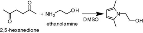
A Paal–Knorr reaction, shown in Scheme 4.3, served as the example chemistry to test the optimization platform using a ReactIR flow cell for quantification of conversion. This reaction, where both the first and second reaction steps affect the overall rate, leads to a more complex conversion profile, although the exact form of the reaction intermediate is still under some debate [45, 46]. The behavior is due to the initial equilibrium step significantly affecting the overall rate of product formation at short reaction times, which leads to a tapered plateau in the reaction production rate. Furthermore, the Paal–Knorr reaction is widely used to form pyrrole rings in synthetic [47, 48] and biological molecules [49, 50] (shown in Schemes 4.3 and 4.4). Additionally, while it is possible to determine conversion based upon advanced chemometrics analysis of the IR spectrum, reaction conversion could be monitored simply by calibration to a single peak height normalized to a single point baseline.

Scheme 4.3 Paal–Knorr reaction [51, 52].

Scheme 4.4 Paal–Knorr reaction mechanism [46, 50, 53].

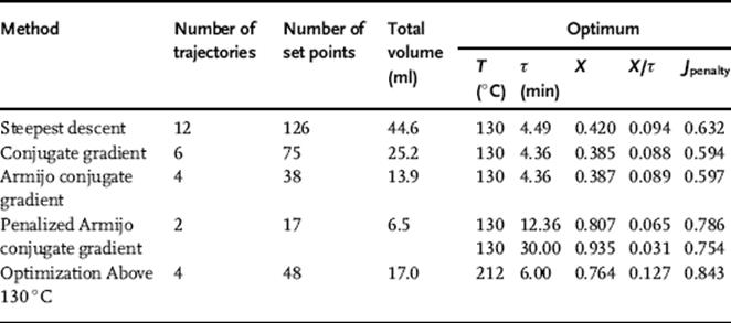
A steepest descent algorithm was first used to optimize production rate (Equation 4.4). The steepest descent algorithm tends to move slowly up the production rate ridge (Figure 4.4a), significantly reducing efficiency. However, this issue was overcome by using a Fletcher–Reeves conjugate gradient method, which found the constrained optimum in much fewer experiments (Figure 4.4b). The conjugate gradient algorithm was then further improved upon by incorporating a hybrid Armijo line search and bisection contraction method (Figure 4.4c). The results of these optimizations are summarized in Figure 4.5 and Table 4.2.

(4.4)

As can be seen in Table 4.2, the conversion, X, was only about 40% at the maximum in production rate. Another optimization was performed using a quadratic loss function to penalize conversions of less than 85% (Figure 4.6). This optimization of production rate led to an optimum at higher residence time, where a conversion of 81% was achieved, demonstrating the tradeoff between conversion and production rate. Because the upper temperature constraint was still active at this optimum, a final optimization was conducted with a significantly higher temperature limit (Figure 4.7).

Figure 4.4 Maximization of the production rate of the Paal–Knorr reaction (Scheme 4.1) with different optimization strategies. Values of the objective function are given by the color bar at right. Control variable boundaries are denoted by dashed red lines. The initial conditions are boxed in black at the bottom left, and the optimum is boxed in red at the top left. The initial DoE of each trajectory is numbered. (a) Steepest descent method. (b) Conjugate gradient method. (c) Armijo conjugate gradient method. Source: Reprinted with permission from the American Chemical Society [39].

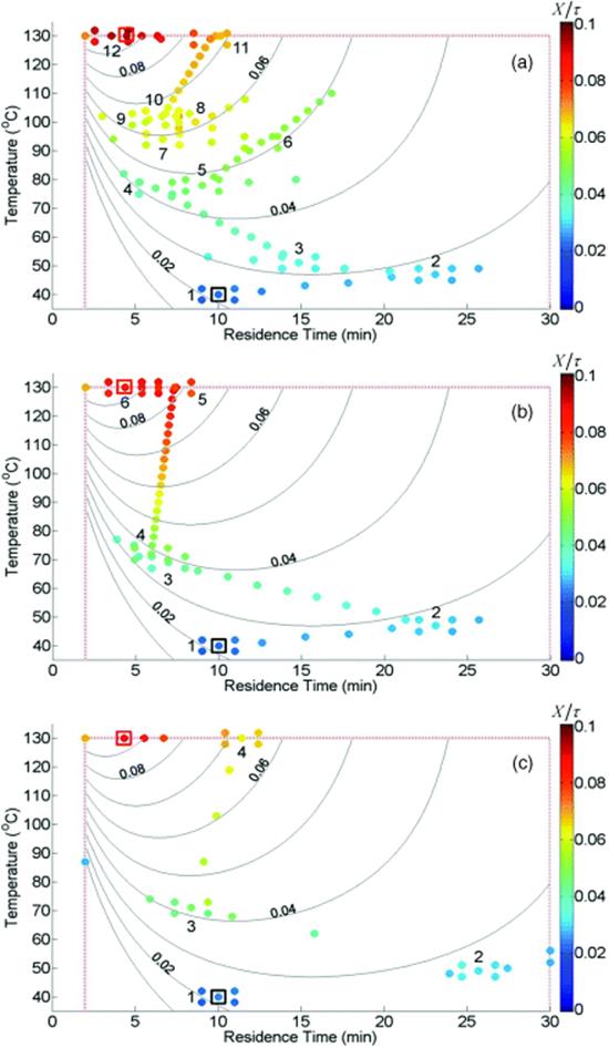
Figure 4.5 Objective function value at each set point for steepest descent (), conjugate gradient (), and Armijo conjugate gradient (). The optimum for each algorithm is boxed. Source: Reprinted with permission from the American Chemical Society [39].

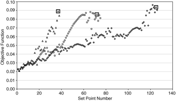
Figure 4.6 Penalized Armijo conjugate gradient method. The conversion (×) and objective function value () at each set point are shown. Values of the objective function are also given by the color bar at right. Control variable boundaries are denoted by dashed red lines. The initial conditions are boxed in black at the top left, and the optimum is boxed in red at the top center. The initial DoE of each trajectory is numbered. Source: Reprinted with permission from the American Chemical Society [39].

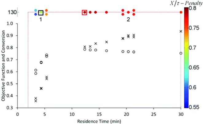
Figure 4.7 Penalized Armijo conjugate gradient method above 130 °C. Values of the objective function are given by the color bar at right. Control variable boundaries are denoted by dashed red lines. The initial conditions are boxed in black at the bottom left, and the optimum is boxed in red at the top left. The initial DoE of each trajectory is numbered. Source: Reprinted with permission from the American Chemical Society [39].

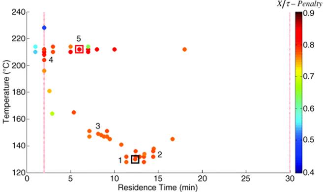
Table 4.2 Summary of optimization algorithm performance.