Physical Chemistry: A Very Short Introduction (2014)
Chapter 1. Matter from the inside
One way to understand how a physical chemist thinks and contributes to chemistry is to start at the interior of an atom and then to travel out into the world of bulk matter. The interior of an atom is where much of the explanation of matter is to be found and it is here that a chemist is most indebted to physics. Within this realm, within an atom, explanations necessarily draw on quantum mechanics, that perplexing description of the behaviour of the very small. That quantum mechanics is central to their description should not be taken to be a warning that the rest of this chapter will be incomprehensible! I shall distil from that theory only the qualitative essence of what we need.
Atoms
The ancient Greeks speculated that matter was composed of atoms. That was pure speculation unsupported by any experimental evidence and so cannot be regarded as the beginning of physical chemistry. Experimental evidence for atoms was accumulated by John Dalton (1766–1844) in the very early 19th century when the use of the chemical balance allowed quantitative measurements to be made on the reactions that matter undergoes. Dalton inferred the existence of atoms from his measurements but had no way of assessing their actual sizes. He had no notion that nearly two centuries later, in the late 20th century, scientists would at last be able to see them.
For a physical chemist, an atom consists of a central, tiny, massive, positively charged nucleus surrounded by a cloud of much lighter, negatively charged electrons. Chemists have little interest in the details of the structure of the nucleus itself and are content to think of it as a tightly bound collection of two types of fundamental particle, positively charged protons and electrically neutral neutrons. The number of protons in the nucleus, the atom’s ‘atomic number’, determines the identity of the element (1 for hydrogen, 2 for helium, and so on up to, currently, 118 for livermorium). The number of neutrons is approximately the same as the number of protons (none for ordinary hydrogen, 2 for ordinary helium, and about 170 for livermorium). This number is slightly variable, and gives rise to the different isotopes of the element. As far as a physical chemist is concerned, a nucleus is a largely permanent structure with three important properties: it accounts for most of the mass of the atom, it is positively charged, and in many cases it spins on its axis at a constant rate.
One particular nucleus will play an important role throughout this account: that of a hydrogen atom. The nucleus of the most common form of hydrogen is a single proton, a single ceaselessly spinning, positively charged fundamental particle. Although so simple, it is of the utmost importance in chemistry and central to the way that physical chemists think about atoms in general and some of the reactions in which they participate. There are two further isotopes of hydrogen: deuterium (‘heavy hydrogen’) has an additional neutron bound tightly to the proton, and tritium with two neutrons. They will play only a slight role in the rest of this account, but each has properties of technical interest to chemists.
The electronic structure of atoms
Physical chemists pay a great deal of attention to the electrons that surround the nucleus of an atom: it is here that the chemical action takes place and the element expresses its chemical personality. The principal point to remember in this connection is that the number of electrons in the atom is the same as the number of protons in the nucleus. The electric charges of electrons and protons are equal but opposite, so this equality of numbers ensures that the atom overall is electrically neutral. Thus, a hydrogen atom has a single electron around its nucleus, helium has two, livermorium has a crowded 118, and so on.
Quantum mechanics plays a central role in accounting for the arrangement of electrons around the nucleus. The early ‘Bohr model’ of the atom, which was proposed by Neils Bohr (1885–1962) in 1913, with electrons in orbits encircling the nucleus like miniature planets and widely used in popular depictions of atoms, is wrong in just about every respect—but it is hard to dislodge from the popular imagination. The quantum mechanical description of atoms acknowledges that an electron cannot be ascribed to a particular path around the nucleus, that the planetary ‘orbits’ of Bohr’s theory simply don’t exist, and that some electrons do not circulate around the nucleus at all.
Physical chemists base their understanding of the electronic structures of atoms on Schrödinger’s model of the hydrogen atom, which was formulated in 1926. Erwin Schrödinger (1887–1961) was one of the founders of quantum mechanics, and in what he described as an episode of erotic passion whilst on vacation with one of his mistresses, he formulated the equation that bears his name and solved it for the location of the electron in a hydrogen atom. Instead of orbits, he found that the electron could adopt one of a variety of wave-like distributions around the nucleus, called wavefunctions, each wave corresponding to a particular energy.
Physical chemists adopt Schrödinger’s solutions for hydrogen and adapt it as the starting point for their discussion of all atoms. That is one reason why the hydrogen atom is so central to their understanding of chemistry. They call the wave-like distributions of electrons atomic orbitals, suggesting a link to Bohr’s orbits but indicating something less well-defined than an actual path.
We shall need some nomenclature. The lowest energy atomic orbital in a hydrogen atom is an example of an s-orbital. An electron in an s-orbital (physical chemists say ‘in’ when they mean having a distribution described by a particular orbital) can be pictured as a spherical cloudlike distribution that is densest at the nucleus and declines sharply with distance from it (Figure 1). That is, the electron is most likely to be found at the nucleus, and then progressively less likely to be found at points more distant from it. Incidentally, an electron in this orbital has no sense of rotation around the nucleus: it is effectively just hovering over and surrounding the nucleus. An atom is often said to be mostly empty space. That is a remnant of Bohr’s model in which a point-like electron circulates around the nucleus; in the Schrödinger model, there is no empty space, just a varying probability of finding the electron at a particular location.
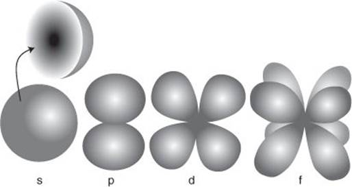
1. The typical shapes of s-, p-, d-, and f-orbitals. The boundaries enclose regions where the electron is most likely to be found. The inset shows the internal structure of an s-orbital, with density of shading representing the probability of finding an electron at each location
There are other s-orbitals, each one of successively higher energy, and each one forming a spherical cloudlike shell at progressively greater distances from the nucleus. They are denoted 1s (the lowest energy s-orbital), 2s, 3s, and so on. In a hydrogen atom only the 1s orbital is occupied by the atom’s lone electron.
There are also other wave-like solutions of the Schrödinger equation for the hydrogen atom (as shown in the illustration). What is called a p-orbital is like a cluster of two clouds on opposite sides of the nucleus, a d-orbital consists of four cloudlike regions, an f-orbital of eight such regions, and so on. There are two points to make in this connection: the s, p, d, f notation is derived from very early spectroscopic observations on atoms and its origin is no longer of any significance except to historians of science, but the notation persists and is a central part of every chemist’s vocabulary. Second, the notation continues to g, h, etc.; but chemists almost never deal with these other orbitals and there is no need for us to consider them further.
Schrödinger went on to show that whereas there is only one way of wrapping a spherical shell around a nucleus (so there is only one s-orbital of any rank), there are three ways of wrapping a p-orbital around the nucleus (so there are three p-orbitals of any rank). Similarly, there are five ways of wrapping the even more complex d-orbitals around the nucleus (five d-orbitals of a given rank) and seven ways of wrapping f-orbitals. Moreover, for a given energy there are only certain types of orbitals that can exist.
The actual pattern is as follows:
1s
2s 2p
3s 3p 3d
4s 4p 4d 4f
and so on, with 1s having the lowest energy.
In a hydrogen atom, all the orbitals of the same rank (the same row in this list) have the same energy. In all other atoms, where there is more than one electron, the mutual repulsion between electrons modifies the energies and, broadly speaking, the list changes to
1s
2s 2p
3s 3p
4s 3d 4p
with more complicated changes in other orbitals. I shall make two points in this connection.
First, physical chemistry has a sub-discipline known as computational chemistry. As its name suggests, this sub-discipline uses computers to solve the very complex versions of the Schrödinger equation that arise in the treatment of atoms and molecules. I shall deal with molecules later; here I focus on the much simpler problem of individual atoms, which were attacked very early after the formulation of the Schrödinger equation by carrying out the enormously detailed calculations by hand. Now atoms are essentially a trivial problem for modern computers, and have been used to derive very detailed descriptions of the distribution of electrons in atoms and the energies of the orbitals. Nevertheless, although physical chemists can now calculate atomic properties with great accuracy almost at the touch of a button, they like to build up models of atoms that give insight into their structure and provide a sense of understanding rather than just a string of numbers. This understanding is then exported into inorganic and organic chemistry as well as other parts of physical chemistry. Models have been built of the way that repulsions between electrons in atoms other than hydrogen affect the order of orbital energies and the manner in which electrons occupy them.
The phrase ‘the manner in which electrons occupy them’ introduces another important principle from physics. In 1925 Wolfgang Pauli (1900–58) identified an important principle when confronted with some peculiar features of the spectroscopy of atoms: he noted that certain frequencies were absent in the spectra, and concluded that certain states of the atom were forbidden. Once quantum mechanics had been formulated it was realized that there is a deep way of expressing his principle, which we shall not use, and a much more direct way for our purposes, which is known as the Pauli exclusion principle:
No more than two electrons may occupy any one orbital, and if two do occupy that orbital, they must spin in opposite directions.
We shall use this form of the principle, which is adequate for many applications in physical chemistry.
At its very simplest, the principle rules out all the electrons of an atom (other than atoms of one-electron hydrogen and two-electron helium) having all their electrons in the 1s-orbital. Lithium, for instance, has three electrons: two occupy the 1s orbital, but the third cannot join them, and must occupy the next higher-energy orbital, the 2s-orbital. With that point in mind, something rather wonderful becomes apparent: the structure of the Periodic Table of the elements unfolds, the principal icon of chemistry.
To see how that works, consider the first 11 elements, with 1 to 11 electrons (the numbers in brackets in this list):
H[1] He[2]
Li[3] Be[4] B[5] C[6] N[7] O[8] F[9] Ne[10]
Na[11]...
(If you need reminding about the names of the elements, refer to the Periodic Table in the Appendix at the end of this volume.) The first electron can enter the 1s-orbital, and helium’s (He) second electron can join it. At that point, the orbital is full, and lithium’s (Li) third electron must enter the next higher orbital, the 2s-orbital. The next electron, for beryllium (Be), can join it, but then it too is full. From that point on the next six electrons can enter in succession the three 2p-orbitals. After those six are present (at neon, Ne), all the 2p-orbitals are full and the eleventh electron, for sodium (Na), has to enter the 3s-orbital. Simultaneously, a new row of the Periodic Table begins. At a blow, you can now see why lithium and sodium are cousins and lie in the same column (‘group’) of the table: each one has a single electron in an s-orbital. Similar reasoning accounts for the entire structure of the Table, with elements in the same group all having analogous electron arrangements and each successive row (‘period’) corresponding to the next outermost shell of orbitals.
This is where physical chemistry segues into inorganic chemistry, the specific chemistry of all the elements. Physical chemistry has accounted for the general structure of the Periodic Table, and inorganic chemistry explores the consequences. It is quite remarkable, I think, that very simple ideas about the existence and energies of orbitals in alliance with a principle that governs their occupation accounts for the brotherhood of the elements, as represented by the Periodic Table.
The properties of atoms
Physical chemists do not quite let slip their grip on atoms at this point and hand them over to inorganic chemists. They continue to be interested in a variety of properties of atoms that stem from their electronic structure and which play a role in governing the chemical personalities of the elements.
Probably the most important property of an atom for the compounds that it can form is its size, specifically its radius. Although an atom has a fuzzy cloud of electrons around its nucleus, the density of the cloud falls off very rapidly at its edge—so speaking of the radius of the atom is not too misleading. In practice, atomic radii are determined experimentally by measuring the distance between two bonded atoms in a molecule or solid, and apportioning the distance to each atom in a prescribed way. The trends in atomic radius are found to correlate with the location of the element in the Periodic Table. Thus, on crossing the Table from left to right, atoms become smaller: even though they have progressively more electrons, the nuclear charge increases too, and draws the clouds in to itself. On descending a group, atoms become larger because in successive periods new outermost shells are started (as in going from lithium to sodium) and each new coating of cloud makes the atom bigger (Figure 2).
Second in importance is the ionization energy, the energy needed to remove one or more electrons from the atom. As we shall see, the ability of electrons to be partially or fully removed from an atom determines the types of chemical bonds that the atom can form and hence plays a major role in determining its properties. The ionization energy more or less follows the trend in atomic radii but in an opposite sense because the closer an electron lies to the positively charged nucleus, the harder it is to remove. Thus, ionization energy increases from left to right across the Table as the atoms become smaller. It decreases down a group because the outermost electron (the one that is most easily removed) is progressively further from the nucleus. Elements on the left of the Periodic Table can lose one or more electrons reasonably easily: as we shall see in Chapter 4, a consequence is that these elements are metals. Those on the right of the Table are very reluctant to lose electrons and are not metals (they are ‘non-metals’).
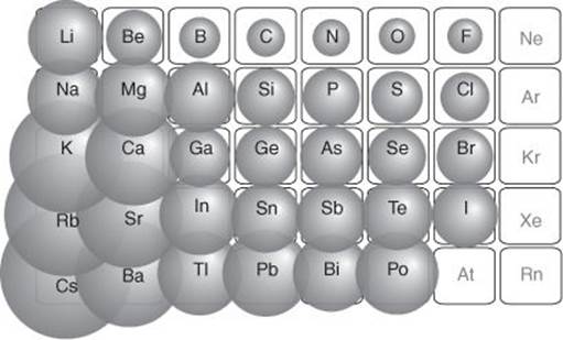
2. The variation in atomic radius across the Periodic Table. Radii typically decrease from left to right across a period and increase from top to bottom down a group. Only the ‘main group’ elements are shown here (not the transition elements)
Third in importance is the electron affinity, the energy released when an electron attaches to an atom. Electron affinities are highest on the right of the Table (near fluorine; ignore the special case of the noble gases). These relatively small atoms can accommodate an electron in their incompletely filled outer cloud layer and once there it can interact strongly and favourably with the nearby nucleus.
The importance of ionization energies and electron affinities becomes apparent when we consider the ‘ions’ that atoms are likely to form. An ion is an electrically charged atom. That charge comes about either because the neutral atom has lost one or more of its electrons, in which case it is a positively charged cation (pronounced ‘cat ion’) or because it has captured one or more electrons and has become a negatively charged anion. The names ‘cation’ and ‘anion’ were given to these ions by physical chemists studying the electrical conductivities of ions in solution, like salt dissolved in water, who noted that one class of ion moved ‘up’ an electrical potential difference and others moved ‘down’ it (‘ion’ comes from the Greek word for traveller, and ‘an’ and ‘cat’ are prefixes denoting ‘up’ and ‘down’, respectively). Elements on the left of the Periodic Table, with their low ionization energies, are likely to lose electrons and form cations; those on the right, with their high electron affinities, are likely to acquire electrons and form anions. This distinction brings us to the heart of one subject explored and elucidated by physical chemists: the nature of the chemical bond.
The ionic bond
A ‘chemical bond’ is what holds neighbouring atoms together to form the intricate structures of the world. All chemical bonds result from changes in the distribution of electrons in the bonded atoms, and so their formation falls very much into the domain of physical chemistry.
Chemists identify three types of bond: ionic, covalent, and metallic. I shall put off the discussion of the metallic bond until Chapter 4 and the discussion of metals. An ionically bonded substance consists of cations and anions clumped together as a result of the attraction between their opposite electric charges. The most famous exemplar of this type of bonding is sodium chloride, common salt, each grain of which consists of a myriad of sodium cations (Na+) clumped together with an equal number of chloride ions (Cl−). ‘Clumping’ is perhaps a misleading term, for the compound is not just a random jumble of ions but serried ranks of them, each Na+ ion being surrounded by six Cl− ions and each Cl− ion likewise surrounded by six Na+ ions in a highly orderly array that extends throughout the little crystal (Figure 3).
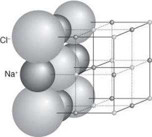
3. The structure of sodium chloride (NaCl). Each sodium ion (Na+) is surrounded by six chloride ions (Cl−), and each Cl− ion is surrounded by six Na+ ions. This pattern is repeated throughout the crystal
Physical chemists identify several significant features of the ionic bond. One is that there is not a discrete ion–ion bond. What I have called ‘clumping together’ is a result of all the ions in the crystal interacting with each other: a Na+ ion interacts favourably with the Cl– ions that surround it, but is repelled by the Na+ ions that surround each of those Cl– ions; in turn it interacts favourably with the next rank of Cl– ions, unfavourably with the next rank of Na+ions, and so on. The attractions and repulsions diminish with distance, but nevertheless ionic bonding should be thought of as a global, not local, aspect of the crystal.
The strength of an ionic bond, and the reason it exists, is that the ions in the crystal have a lower energy than the same number of widely separated sodium and chlorine atoms. This is where ionization energies and electron affinities come into play to determine whether bond formation is favourable. Here, physical chemists turn into profit-and-loss accountants. At first sight the balance sheet shows loss rather than profit. The ionization energy of sodium is low, but its single outermost electron doesn’t simply fall off: there is a substantial energy investment needed to remove it. That investment is partly recovered by the electron affinity of chlorine, with energy released when the electron attaches to a chlorine atom to form Cl–. However, that overall process still requires energy because the energy lowering that occurs in the second step is much less than the energy required in the first ionization step. The additional release of energy that turns loss into profit is the very strong net favourable interaction between the ions that are formed, and which is released as they clump together. In effect, this huge lowering of energy drags the ions into existence and results in a stable crystal of sodium chloride.
You can now see a third characteristic of ionic bonds: that they form primarily between atoms on the left and right of the Periodic Table. Atoms on the left have low ionization energies, so the energy investment for forming cations is reasonably low. Atoms on the right have reasonably high electron affinities, so there is a reasonable lowering of energy when they form anions. This net loss (it is always a loss, for ionization energies are high and electron affinities not very helpful) is turned into profit by the resulting global net attraction between the ions.
The covalent bond
Elements on the right of the Periodic Table have such high ionization energies that if they alone are involved in bond formation, then loss is never turned into profit. Physical chemists have identified another way in which atoms can form liaisons with one another, especially if like elements towards the right of the Table they are reluctant to release electrons and form cations. These atoms compromise: they share their electrons and form what is known as a covalent bond.
I need to step back a little from this development before explaining the concept and consequences of covalent bonding, and make a couple of points. First, the significance of the ‘valent’ part of covalent. This term is derived from the Latin word for ‘strength’ (‘Valete!’, ‘Be strong!’, was the Roman farewell); the word valence is now a common chemical term in chemistry referring to the theory of bond formation. The ‘co’ part is an indication of cooperation between atoms for achieving bond strength.
Second, it is hard to pinpoint the moment in history when physical chemistry became an identifiable discipline within chemistry. There were certainly physical chemists in the 19th century: Michael Faraday among them and Robert Boyle (Chapter 4) even earlier in the 17th century, even though they did not use the term. However, one branch of physical chemistry did emerge right at the beginning of the 20th century when the electron (discovered in 1897) became central to chemical explanation, and perhaps a good starting point for this branch of the discipline is the identification of the covalent bond. That identification is due to the American chemist Gilbert Lewis (1875–1946), who proposed in 1916 that the covalent bond is a shared pair of electrons. It is one of the scandals of intellectual history that Lewis never received the Nobel Prize despite his several seminal contributions to chemistry and physical chemistry in particular.
As I have indicated, a covalent bond is a shared pair of electrons. If an atom has too high an ionization energy for cation formation to be energetically feasible, it might be content to surrender partial control of an electron. Moreover, it might recover some of that small energy investment by accommodating a share in an electron supplied by another like-minded atom provided that overall there is a lowering of energy. I have purposely used anthropomorphic terms, ‘content to’ and ‘like-minded’, for they commonly creep into chemists’ conversations as shorthand for what they really mean, which is an allusion to the changes in energy that accompany the redistribution of electrons. I shall avoid them in future, for they are sloppy and inappropriate (but often whimsically engaging, and like much conversational informality, help to avoid pedantic circumlocutions).
The principal characteristic of covalent bonding is that, in contrast to ionic bonding, it is a local phenomenon. That is, because the electrons are shared between neighbours, an identifiable bond exists between those two neighbours and is not distributed over myriad ions. One consequence of this local character is that covalently bonded species are discrete molecules, like hydrogen, H2 (H—H), water, ![]() , and carbon dioxide, CO2 (O ═ C ═ O). I use these three molecules as examples for a particular reason.
, and carbon dioxide, CO2 (O ═ C ═ O). I use these three molecules as examples for a particular reason.
First, H2 reveals that atoms of the same element might bond covalently together. Such forms of the elements are common among the non-metals (think of oxygen, O2, and chlorine, Cl2). The formula H—H also shows how chemists denote covalent bonds: by a dash between the linked atoms. Each such dash indicated a shared pair of electrons. The water molecule is H2O; I have included it both to show that not all the electrons possessed by an atom need be involved in covalent bond formation and that by forming two bonds the oxygen atom is surrounded by eight electrons (four pairs). The unused pairs are called lone pairs. The fact that eight electrons are present indicates that the oxygen atom has gone on to form as many bonds as it can until it has completed what we have already seen as the capacity of its outermost cloud of electrons. This so-called ‘octet formation’ is one of the guiding but not always reliable principles of bond formation. Finally, I have included carbon dioxide because it shows that more than one pair of electrons can be shared between two atoms: the = indicates a ‘double bond’, consisting of two shared pairs of electrons. There are also molecules with triple bonds (three shared pairs), and very occasionally quadruple bonds.
Not all covalently bonded species are discrete molecules. It is possible in some instances for covalent bond formation to result in extended networks of bonds. The most famous example is diamond, where each carbon atom is singly-bonded to four neighbours, and each of those neighbours bonded to their neighbours, and so on throughout the crystal. I shall return to a discussion of these structures in Chapter 4.
The quantum mechanics of bonds
Although he developed several speculative fantasies, Lewis had no idea of the real reason why an electron pair is so central to covalent bond formation. That understanding had to await the development of quantum mechanics and its almost immediate application to valence theory. That green shoot of an application has since evolved into a major branch of physical chemistry namely theoretical chemistry or, more specifically for those dealing with numerical calculations, computational chemistry.
Physical chemists, initially in collaboration with physicists, have developed two quantum mechanical theories of bond formation, valence-bond theory (VB theory) and molecular orbital theory (MO theory). The former has rather fallen out of favour but its language has left an indelible mark on chemistry and chemists still use many of its terms. MO theory has swept the field as it has proved to be much more readily implemented on computers. Because VB theory language is still used throughout chemistry but calculations are carried out using MO theory, all chemists, under the guidance of physical chemists, need to be familiar with both theories.
VB theory was formulated by the physicists Walter Heitler (1904–81), Fritz London (1900–54), and John Slater (1900–76) and elaborated by the chemist Linus Pauling (1901–93) almost as soon as quantum mechanics had been born, in 1927. This collaboration of physicists and chemists is an excellent example of the foundation that underlies physical chemistry: it also illustrates the intellectual fecundity of youth, as all its originators were in their 20s. The core idea of VB theory is that a wavefunction can be written for the pair of electrons that form a bond. The reason for the importance of the pair being that each electron has a spin (as I mentioned when discussing atoms) and for that bond wavefunction to exist the two electrons must spin in opposite directions. Note that this description focuses on neighbouring pairs of atoms: one atom provides an electron that spins clockwise, the other atoms provides an electron that spins counterclockwise, and the two electrons pair together. Close analysis of the resulting wavefunction shows that this pairing allows the two electrons to accumulate between the two nuclei and, through their electrostatic attraction for the nuclei, effectively glue the two atoms together.
The theory quickly ran into initial difficulties with carbon and its fundamental compound, methane, CH4. This is one place where Pauling made his principal contribution and where the language he introduced survives to pervade modern chemistry. The lowest energy state of a carbon atom has four electrons in its outermost cloud (its ‘valence shell’), two of which are already paired. The remaining two can pair with electrons provided by two hydrogen atoms, but that results in CH2, not CH4. Pauling proposed the idea of promotion, in which it is envisaged that there is a notional energy investment in transferring one of the paired 2s electrons into an empty 2p-orbital. Now all four electrons can be available for pairing with electrons providing by hydrogen atoms, so allowing the formation of CH4.
Promotion, however, raises another problem, for one of the bonds (the one involving the original 2s-orbital) is different from the other three (formed by pairing with electrons in the three 2p-orbitals), but in CH4 all four bonds are known to be the same. Pauling overcame this problem by proposing the concept of hybridization. Each 2s-and 2p-orbital is like a wave centred on the nucleus: like all waves they can be considered to interfere if they occupy the same region of space, which in this atom they do. Analysis of the interference between the four waves shows that they result in four interference patterns that correspond to orbitals that are identical except for pointing in different directions (to the corners of a tetrahedron in this case). These ‘hybrid orbitals’, Pauling proposed, should be used to form the covalent bonds of the CH4 molecule. The result is four identical bonds and a molecule that looks like a miniature tetrahedron, exactly as is observed.
Another simple molecule, hydrogen chloride (HCl) presented another problem, for analysis of the VB wavefunction showed that it was a poor description of the distribution of electrons in one important respect: it never allowed both electrons to be on the chlorine atom at the same time. We have seen that chlorine, on the right of the Periodic Table, has a high electron affinity, so it is physically implausible that the two electrons of the bond don’t spend a good proportion of their time close to it. Here Pauling proposed the concept of resonance. Instead of writing a single wavefunction representing an H–Cl molecule, another one should be written for a tiny (and in this case, local) ionic structure, H+Cl−, and both should contribute to the actual structure of the molecule. This so-called ‘superposition’ of wavefunctions, allowing both to contribute to the description, is called resonance, and its inclusion improves the description of the molecule (and results in a lower calculated energy: always a sign of improvement).
Resonance was simultaneously the saviour and the cause of the downfall of VB theory. It saved the day for small molecules, where there are only a few resonance structures to consider, but it proved an insurmountable barrier for big molecules where thousands of structures could contribute to the resonance.
MO theory was initially formulated by Robert Mulliken (1896–1986) and Friedrich Hund (1896–1997) in 1927 as a rival to VB theory; the name was coined by Mulliken in 1932. It can be regarded as a natural extension of the theory of the electronic structure of atoms. As we have seen, in an atom electrons occupy (that is, have distributions described by) wavefunctions called atomic orbitals. In a molecule, according to MO theory, electrons occupy wavefunctions called ‘molecular orbitals’ that spread over all the nuclei present in the molecule and help bind them together into a stable arrangement. According to the Pauli exclusion principle, each molecular orbital, like an atomic orbital, can accommodate no more than two electrons and their spins must be paired, so immediately the importance of Lewis’s electron pairing is explained.
The Schrödinger equation for molecular orbitals is far too difficult to solve, so approximations are essential. First, molecular orbitals are constructed from all the atomic orbitals that are present in the molecule. Thus, in H2, the two 1s atomic orbitals are used. As for any waves, interference occurs where these wavefunctions spread into the same region of space (as mentioned in the discussion of hybridization, but here it is interference between waves centred on neighbouring atoms). In this case, the interference may either enhance the amplitude of the waves where they overlap or diminish it. The former gives rise to a bonding orbital, for electrons that occupy it will be found accumulated between the two nuclei and glue them together by the attraction between opposite charges. Destructive overlap results in a reduction in amplitude of the wavefunction between the two nuclei and thus removes the electrons from where it is beneficial for them to be. The combination is therefore called an antibonding orbital, as electrons in it tend to drive the nuclei apart (Figure 4).
Although the Schrödinger equation is too difficult to solve for molecules, powerful computational procedures have been developed by theoretical chemists to arrive at numerical solutions of great accuracy. All the procedures start out by building molecular orbitals from the available atomic orbitals and then setting about finding the best formulations. This branch of physical chemistry is the subject of intense development as the power of computers increases. Depictions of electron distributions in molecules are now commonplace and very helpful for understanding the properties of molecules. It is particularly relevant to the development of new pharmacologically active drugs, where electron distributions play a central role in determining how one molecule binds to another and perhaps blocks the deleterious function of a dangerously invasive molecule.
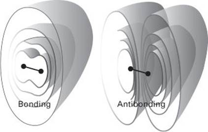
4. The bonding and antibonding orbitals in a two-atom molecule. In a bonding orbital, the electrons accumulate between the two nuclei and bind them together. In an antibonding orbital, they are excluded from the internuclear region and the two nuclei push each other apart. Similar comments apply to molecules composed of many atoms. The surfaces are contours of equal probability for finding the electron
These computational procedures fall into three broad categories. The semi-empirical procedures acknowledge that some computations are just too time-consuming (and therefore expensive) unless some of the parameters needed in the calculations are taken from experiment. The purer ab initio (‘from scratch’) procedures stand aloof from this compromise, and seek to perform the calculation with no input other than the identities of the atoms present. Initially only small molecules could be treated in this way, but as computational power increases so larger and larger molecules are captured in its net. One currently fashionable procedure is a blend of these approaches: density functional theory is widely applicable as it provides a swift and reasonably accurate way of calculating the properties of a wide range of molecules.
The current challenge
Bond formation is essentially fully understood apart from some recondite questions relating to the role of the contributions of potential and kinetic energy and to the presence of relativistic effects in heavy atoms. The principal focus now is on the efficient and reliable computation of the electronic structures of ever bigger molecules, including biologically interesting molecules, the electronic properties of nanostructures, and detailed descriptions of the behaviour of electrons in molecules. Chemical reactions are increasingly being modelled computationally, with insight being gained into how bonds are broken and new ones formed. Drug discovery, the identification of pharmacologically active species by computation rather than in vivo experiment, is an important target of modern computational chemistry.