Physical Chemistry Essentials - Hofmann A. 2018

Mixtures and Phases
3.4 Thermodynamic Aspects of Phase Transitions

The locations of phase boundaries (lines) in phase diagrams are determined by the relative thermodynamic stability of the individual phases, i.e. by the chemical potential μ (molar Gibbs free energy G _m). The chemical potential can thus be thought of as the potential of a substance to bring about a physical change. Under different conditions, different forms of the same system become more stable. A system that is in equilibrium has the same chemical potential throughout in all actually existing phases at that time.

In this section, we will discuss how the stability of phases are affected by particular environmental conditions. Knowledge about these relationships will allow us to predict phase transitions based on thermodynamic parameters.

3.4.1 Temperature Dependence of Phase Stability

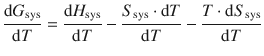
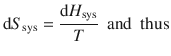
We have previously (2.2.1) learned that the Gibbs free energy of a system is given by:

(2.44)

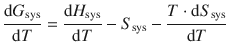
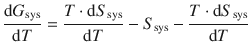
and thus its derivative is calculated as per

(2.45)

which can be resolved by considering the product rule (A.2.3):

After dividing the equation by dT, one obtains:

which simplifies to:

(3.15)

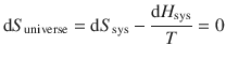
In Sect. 2.2.2, it was established that for processes at equilibrium, there is no net change in the entropy of the universe:

(2.51)

The entropy of the universe was given by Eq. 2.47:

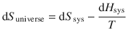
which combines to:

From this equation, it follows that

We can now use this expression to substitute dH _sys in Eq. 3.15 and obtain:

which simplifies to

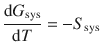
(3.16)

When considering a system consisting of 1 mol of substance (so we can use G _m = μ), and remembering that the Gibbs free energy is not only dependent on the temperature, but also on the pressure, we obtain the following expression from Eq. 3.16 and also introduce the molar entropy S _m:

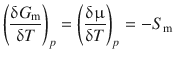
(3.17)

Since G (as well as G _m, μ) is also dependent on the pressure, we need to request constant pressure when calculating the temperature differential; this is done by calculating a partial differential (indicated by ’δ’), and denoting the pressure as a subscript.

The molar entropy S _m is a characteristic parameter of a substance and always positive. Therefore, the change of the chemical potential μ with increasing temperature at constant pressure is always negative.

The phase with the lowest chemical potential μ at a particular temperature is the most stable one for that temperature. The transition temperatures (T _m/T _f and T _b) are the temperatures, at which the chemical potentials of the two interfacing phases are equal and the phases are thus at equilibrium.

3.4.2 Entropies of Substances

In the previous section, we have introduced the molar entropy S _m in the context of different phases of a one-component system. We also noted that molar entropies are characteristic parameters of a substance.

In gases, molecules can freely diffuse through the volume they are contained in and the individual molecules (as well as their energies) are dispersed across the entire volume. Therefore, the degree of disorder is rather large, compared to that of liquids or solids. The molar entropy S _m of gases is thus larger than that of liquids or solids (see Table 3.2).

Table 3.2

Molar entropies S _m in J K⁻¹ mol⁻¹ of selected solids, liquids and gases at 25 °C

In contrast, the molecules in a solid are confined to a small volume and their degrees of freedom are restricted to vibrational motion. The molar entropies S _m of solids are thus fairly low. Solids comprising of large molecules (e.g. sucrose) or complexes (CuSO₄·5 H₂O) have a large number of atoms and may thus possess comparatively high molar entropies, since the energy may be shared among the many atoms.

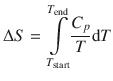
We remember that we have defined the explicit entropy change dS in Sect. 2.1.10 as:

(2.30)

where dQ is the reversibly transferred heat at a particular temperature T. From this equation, it becomes clear that there is a smaller change of entropy when a given quantity of energy (dQ) is transferred to an object at high temperature than at low temperature. More disorder is induced when the object is cool rather than hot.

The ability of a substance to distribute energy over its molecules is related to the heat capacity. As we have discussed in Sect. 2.1.12, this link can be used to establish a relationship between the entropy change and the heat capacity C _p :

(2.39)

which forms the basis for entropy determination of substances by heat capacity measurements (i.e. calorimetrically). Alternatively, electrochemical cells can be used to determine entropies of substances.

3.4.3 Pressure Dependence of Melting

In Sect. 4.1 above, we looked at the change of the Gibbs free energy with temperature (at constant pressure) and derived the definition of the molar entropy S _m. From the Maxwell equations describing the relations between different state variables (Sect. 2.1.14), the variation of the Gibbs free energy with pressure (at constant temperature) can be derived, leading to the definition of the molar volume V _m:

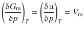
(2.65)

Like the molar entropy, the molar volume V _m is a characteristic parameter for a substance and always positive. Therefore, the change of the chemical potential μ (= G _m) with increasing pressure at constant temperature is always positive. Generally, the molar volume V _m is larger for liquids than for solids (exception: water).

We remember that the transition temperatures (T _m/T _f and T _b) are the temperatures, at which the chemical potentials of the two interfacing phases are equal and the phases are thus at equilibrium. The transition temperature between the solid and liquid phases (T _m/T _f) is generally larger at higher pressures (exception: water).

Conceptually, this is illustrated in Fig. 3.11. If the molar volume V _m of the solid is smaller than that of the liquid (Fig. 3.11 left)—an observation made for most substances—the chemical potential of the solid phase μ_(s) increases less than the chemical potential of the liquid phase, μ_(l), when the pressure is increased. This situation leads to a shift of the intersect between the two branches to higher temperatures; therefore, the melting temperature increases when the pressure is increased.

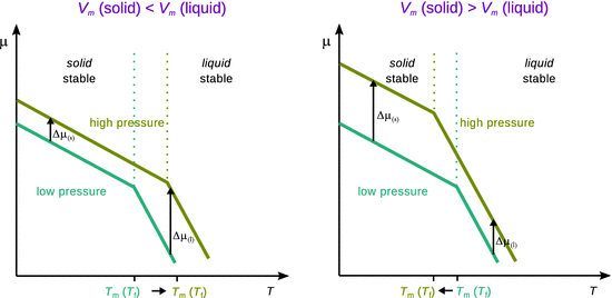
Fig. 3.11

The blue and green lines show the chemical potential in dependence of the temperature. The branch at lower temperature describes the chemical potential for the solid and the branch at higher temperature describes the chemical potential for the liquid phase. The transition temperature is the temperature where the two branches intersect. An increase of the chemical potential (when the pressure is increased) results in a vertical shift of the branches. The phase with the smaller volume is less impacted by a change of pressure and thus has a lesser change of the chemical potential

In contrast, water, for example, shows the behaviour illustrated in the right panel of Fig. 3.11: the molar volume V _m of the solid is larger than that of the liquid. Therefore, when the pressure is increased, the liquid phase experiences a lesser change of the chemical potential than the solid phase. The intersect between the two branches thus migrates to lower temperatures. This means that at higher pressure, substances like water freeze at lower temperatures.

3.4.4 Pressure Dependence of Vapour Pressure

In Sect. 3.2.2, we arrived at an expression of Raoult’s law that relates the vapour pressure of a solution with that of the pure solvent as per:

(3.11)

μ_A(l) and describe the chemical potentials of the solution and the pure solvent, respectively. In the previous section, we have seen that the differential of the chemical potential with respect to pressure changes is

(2.65)

We then realise that the chemical potential difference in Eq. 3.11 can be expressed in terms of the molar volume and the pressure change:

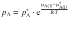
which we can substitute in Eq. 3.11 and obtain:

(3.18)

The pressure difference Δp in the exponential term describes the pressure of two different states. Let the initial state be at p _initial = p^—, and the final state at a much high pressure. In that case, Δp > 0 and thus the exponent is positive and the entire exponential term a factor greater than 1 (see Fig. 3.12). This means that the vapour pressure of a pressurised liquid is higher than that of the system under standard pressure.

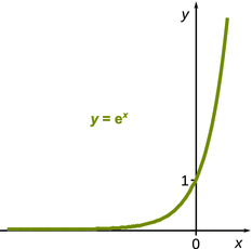
Fig. 3.12

For positive arguments x, the function y = e ^x yields values larger than 1. For negative arguments, the function yields values less than 1

Similarly, if we consider the case where p _final describes the system at lower pressure (e.g. the evacuated system), then we appreciate that Δp < 0, the exponent becomes negative and thus the exponential factor has a value less than 1. Therefore, the vapour pressure will be less in an evacuated system than in one that contains ambient atmosphere.

3.4.5 Phase Boundaries

As we have established earlier, the lines in a phase diagram separating two neighbouring phases are called phase boundaries. Along those boundaries, two phases (we will here call them ’a’ and ’b’) co-exist. Being lines in a two-dimensional plot, the phase boundaries are best discussed in terms of their slopes. So for a p-T diagram, phase boundaries are characterised by the differential

Since the two phases co-exist, there must be equilibrium and the changes in the chemical potentials must be equal:

From earlier discussions we know that

(2.45)

and can therefore substitute this expression on both sides of the equilibrium equation above:

We group together the volumes and entropies on opposing sides:

and consider that the differences of the volumes and entropies of phases ’a’ and ’b’ describe the transition from one phase to the other:

This equation can be re-arranged to yield the slope of the phase boundary through the differential of pressure and temperature:

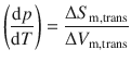
(3.19)

This equation is of fundamental importance as it describes the phase transitions (phase boundaries) in p-T phase diagrams; it is also known as the Clapeyron equation, developed by the French physicist an engineer Benoît Clapeyron in 1834 (Clapeyron 1834). Equipped with this equation, we can now discuss the three phase boundaries solid—liquid, liquid—vapour and solid—vapour.

3.4.6 Phase Boundaries: Solid—Liquid

We can apply the general form of the Clapeyron equation above to particular phase transitions, such as the melting or fusion process where solid and liquid phases are in equilibrium. The slope of the solid—liquid phase boundary in a p-T diagram is described as the differential of pressure (y-axis) with respect to temperature (x-axis), . The differences in the molar entropies and volumes between solid and liquid states are macroscopically measurable; we thus use ’Δ’ instead of ’d’, and obtain the Clapeyron equation for the melting (fusion) process:

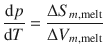
(3.19)

We remember from earlier discussions that

(2.35)

and therefore can express the phase transition in terms of the molar enthalpy change:

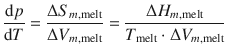
(3.20)

For the melting process, we can evaluate the Clapeyron equation in an approximative fashion. The change in molar enthalpies

is generally positive, and the change in molar volumes

is generally positive and rather small (the liquid and solid states of most substances have a similar volume, with the liquid phase typically having a slightly larger volume; exception: water). Also, ΔV _m,melt can be considered independent of the temperature. Therefore, the differential

is generally positive and large. This means we will obtain steep boundaries at the solid—liquid interfaces in a p-T diagram (Fig. 3.13), with this phase boundary having a positive slope.

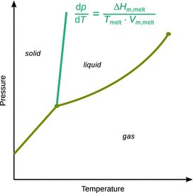
Fig. 3.13

Using the Clapeyron equation, the slope of the phase boundary between solid and liquid phases can be calculated. Most substances have a lesser density in their liquid than in their solid states, hence the molar volume difference upon melting is positive, and the phase boundary therefore has a positive slope

3.4.7 Phase Boundaries: Liquid—Vapour

In analogy to the discussion in the previous section, we can formulate, based on the Clapeyron equation, an expression for the vapourisation process, i.e. the transition from the liquid to the gas phase:

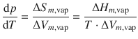
(3.19)

For the vapourisation process, we can not assume that ΔV _m,vap is independent of the temperature. We remember that for an ideal gas, there is a relationship between the gas volume and the temperature and pressure, given by the ideal gas equation:

(2.6)

When we consider the molar volume V _m , we normalise the volume with respect to the molar amount n (), so we obtain:

Since the gas phase of a substance occupies a much larger volume than the liquid state, we can assume that the volume of the liquid is negligible compared to the volume of the gas:

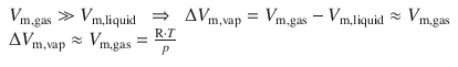
Note that we now assume conditions of an ideal gas and negligible volume of the solid compared with the gas. This expression for ΔV _m,vap can be used to substitute in Eq. 3.19 which then yields:

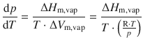
This simplifies to

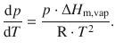
We isolate the two independent variables, p and T, on opposite sides of the equation, and use the formality of to achieve a more convenient notation (see Appendix A.3.1). This results in a relationship known as the Clausius-Clapeyron equation:

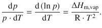
(3.21)

This equation was first derived by the German physicist and mathematician Rudolf Clausius in 1850 (Clausius 1850).

3.4.8 Phase Boundaries: Solid—Vapour

The phase boundary between the solid and vapour phases describes the sublimation (or deposition) process. For this process, the Clapeyron equation yields:

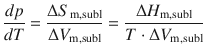
(3.19)

As in the vapourisation process (previous section), we can not assume that ΔV _m is independent of the temperature, because a gas phase is involved. Therefore, we again replace V _m with the expression from the ideal gas equation. We thus assume conditions of an ideal gas and negligible volume of the solid compared with the gas. The substitution yields:

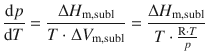
Which simplifies to the following equation, also called the Clausius-Clapeyron equation for the sublimation process:

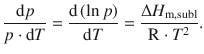
(3.22)

3.4.9 The Ehrenfest Classifications

In Fig. 3.11, we visualised the change of the chemical potential μ with temperature in the region where the solid—liquid phase transition occurs. At the transition, the chemical potential function shows a kink (the function is continuous, but the first derivative of the function is not), so the change in the chemical potential μ is not smooth with a change in the temperature T. This is observed at all major phase transitions

✵ solid↔liquid (melting/freezing)

✵ liquid↔gas (vapourisation/condensation)

✵ solid↔gas (sublimation/deposition)

which are therefore called first order phase transitions. At a molecular level, first-order transitions involve the relocation of atoms, molecules or ions, accompanied by a change of the interaction energies.

What is the implication of this for material properties? As mentioned above, a mathematical function with a kink is characterised by an abrupt change of direction of the plotted function. Whereas the function is continuous and possesses discrete values all the way along, the first derivative is discontinuous. At the kink, the first derivative is infinite.

We remember that the Clapeyron equation (3.19, 3.20) is a function of enthalpy and temperature, in fact , and the first derivative of this function, , leads us to the heat capacity for constant pressure, C _p :

(2.29)

At a first-order transition, H changes by a finite amount whereas T changes by an infinitesimal small amount. The heat capacity C _p (the first derivative) thus becomes infinite.

Following this classification concept, a transition for which the first derivative of the chemical potential μ with respect to the temperature T is continuous, but the second derivative is discontinuous, is called second order phase transition. This implies that volume, entropy and enthalpy do not change at the transition. The heat capacity C _p is discontinuous but not infinite. At a molecular level, second-order transitions are often associated with changes of symmetry in a crystal structure. Rather than the molecular interaction energies, it is the long-range order that varies. Examples for second order phase transitions include the conducting-superconducting transition in metals at low temperatures.

Phase transitions that are not first order, but where nevertheless the heat capacity C _p becomes infinite, are called λ-transitions. In such instances, the heat capacity typically increases well before the actual transition occurs. At a molecular level, λ-transitions are associated with order-disorder transitions. Examples include:

✵ order-disorder transitions in alloys

✵ onset of ferromagnetism

✵ fluid-superfluid transition in liquid helium (hence the name λ-line in the He phase diagram, Fig. 3.9)