Physical Chemistry Essentials - Hofmann A. 2018

Mixtures and Phases
3.5 Mixtures of Volatile Liquids

3.5.1 Phase Diagrams of Mixtures of Volatile Liquids

We assume a mixture of two volatile liquids, A and B, where the liquid and vapour phases are in equilibrium. Even though, the compositions in the two phases are not necessarily the same; the vapour phase will contain more of the more volatile component.

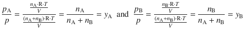
Raoult’s law enables calculation of the vapour pressure of a particular liquid (A) in a mixture, for different concentrations of that liquid in the mixture (expressed as molar fraction x):

(3.11)

is the vapour pressure of the pure liquid A (i.e. at x _A = 1). Since we will have to consider mole fractions for several different phases in the following discussion, in this current chapter, we will denote the mole fraction of substances in the liquid phase as ’z’ instead of ’x’.

The total vapour pressure in an ideal mixture of A and B is then given by Dalton’s law (Eq. 2.8), which poses that the total vapour pressure of a vapour mixture is the sum of the partial vapour pressures of all components (here, the partial vapour pressures are given by Raoult’s law for A and B):

(3.23)

where z _A and z _B are the mole fractions of A and B in the liquid, and and the vapour pressures of the pure liquids, respectively. This relationship may be plotted in a diagram (see Fig. 3.4, upper left) where the total pressure p provides the ordinate (y-axis) and the mole fraction z _A the abscissa (x-axis). It is obvious, that at z _A = 0, there is pure liquid B and hence the total vapour pressure is given by the vapour pressure of pure liquid B, .

With Dalton’s law informing us that the total pressure of a gas mixture equals the sum of the partial pressures of the individual components, we have access to the mole fraction of the individual components in the vapour phase, which, for clarity, we call ’y’ instead ’x’ in this section:

(3.24)

y _A and y _B are the mole fractions of A and B in the vapour. This relationship may also be plotted in a phase diagram (Fig. 3.14, upper right) with pressure as the ordinate (y-axis), but this time the mole fraction y _A as abscissa (x-axis). It is no surprise that the resulting phase boundary is now a different line than before; after all we are no longer plotting against the mole fraction of A in the liquid, but in the vapour. From Eq. 3.24 it is obvious that at y _A = 1, the vapour contains pure substance A, hence the total vapour pressure p is the vapour pressure of A, .

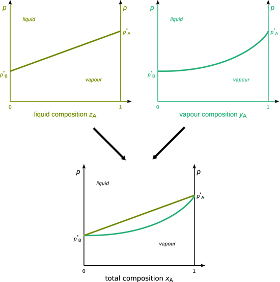
Fig. 3.14

Concept of a binary p-x phase diagram. The phase diagram plotting total composition as the abscissa can be thought of as a superposition of phase diagrams for liquid and vapour composition

Equipped with these relationships, we can now calculate the mole fraction of each component in the vapour phase (y _i ) of the liquid mixture, knowing their mole fractions in the liquid phase (z _i ).

From Raoult’s law we know:

and from Dalton’s law:

Therefore:

For a mixture consisting of two components only, the mole fraction of the second component is then available as

From a practical perspective, it will be very inconvenient to plot two phase diagrams, one each for liquid and vapour mole fractions. Hence the two diagrams are combined into one (Fig. 3.14, bottom).

The combined phase diagram is plotted with the pressure as ordinate and the mole fraction of the total composition as abscissa. The mole fraction of the total composition (x _i ) can easily be obtained from the mole fractions in the liquid (z _i ) and vapour phases (y _i ); an example is shown in Table 3.3.

Table 3.3

Example calculation to obtain the total composition of a binary system, when the compositions of liquid and vapour phases are known

From binary phase diagrams such as the one shown in Fig. 3.15, composition data of the system at various conditions can be easily obtained.

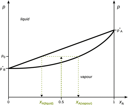
Fig. 3.15

Illustration of how to obtain molar compositions of liquid and vapour phases of a binary liquid mixture

For example, a mixture of two liquids A and B, each present with a mole fraction of 0.5 and a phase diagram as shown in Fig. 3.15 is held at a pressure p = p ₀. In the diagram this situation is depicted as a point at (x _A; p) = (0.5; p ₀). This point lies in the region between the two lines marking the liquid—vapour phase boundary; the upper line which delivers the molar composition of the liquid phase and the lower line which represents the composition of the vapour phase. This area is called the two-phase area, where the liquid and vapour phases co-exist. Therefore, at the identified point, a line parallel to the x-axis is used to extrapolate to the phase boundary lines (such a line is called a conode or tie line). Where the tie line intersects, drop lines to the x-axis are used to determine the molar fraction of A in the vapour and liquid phases. The molar fractions for B are available as per:

As a result of the mixing with substance B, the vapour pressure of A in the mixture is lowered as compared to the vapour pressure of pure liquid A. The mole fraction of A in the vapour phase of a 1:1 mixture is therefore larger than 50%, despite it possessing the higher vapour pressure when comparing the pure liquids.

Any point located in the two-phase indicates a mixture composition where separation into the two co-existing phases occurs. The tie line further yields information about the relative molar amounts of substance A (since x _A is plotted as abscissa) in the liquid and vapour phases. The ratio of molar amounts of substance A in the liquid and vapour phases is given by the lever rule, graphically illustrated in Fig. 3.16:

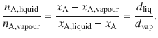
(3.25)

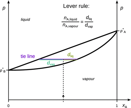
Fig. 3.16

Illustration of the lever rule to determine the molar amounts of substance A in the liquid and vapour phases

The examples and illustrations above were all concerned with pressure-composition (p-x) phase diagrams, where phase boundaries are characterised in dependence of pressure at a particular constant temperature.

Of practical importance are also temperature-composition (T-x) phase diagrams, which show phases at a single pressure. A typical T-x diagram found with many real mixtures is shown in Fig. 3.17. The way of determining the mole fractions of a substance in the liquid and vapour phases in T-x diagrams is the same as discussed above for p-x diagrams. The lever rule can also be applied in an analogous fashion.

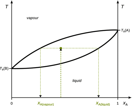
Fig. 3.17

Illustration of how to obtain molar compositions of liquid and vapour phases of a binary liquid mixture from a T-x phase diagram. The process is the same as described above for p-x diagrams. However, note that the location of liquid and vapour phases in T-x diagrams is different to those in p-x diagrams

Temperature-composition phase diagrams are particularly useful when analysing distillation processes.

3.5.2 Simple Distillation

Distillation procedures are based on vapour and liquid having different compositions. In a simple distillation apparatus, mixtures comprising two components of low (component A) and high (component B) volatility can be separated to some degree. Since the distillation experiments are carried out at constant pressure (ambient pressure or under vacuum), temperature-composition phase diagrams such as the one shown in Fig. 3.18, can be used to track the process of simple distillation.

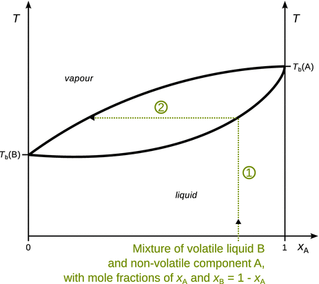
Fig. 3.18

Illustration of a simple distillation process

We are starting at ambient temperature with a liquid mixture that has relatively low concentration of the high volatility component B (x _A ≈ 0.75, so x _B ≈ 0.25). The mixture is heated (arrow 1), and at the intersection of arrow 1 with the boiling curve a vapour phase appears. The composition of the vapour can be obtained where the tie line (arrow 2) intersects with the condensation curve. In a basic distillation apparatus, vapour with this composition is condensed on the fractionation side of the apparatus; the condensate consists of a liquid with enriched component B (Fig. 3.19).

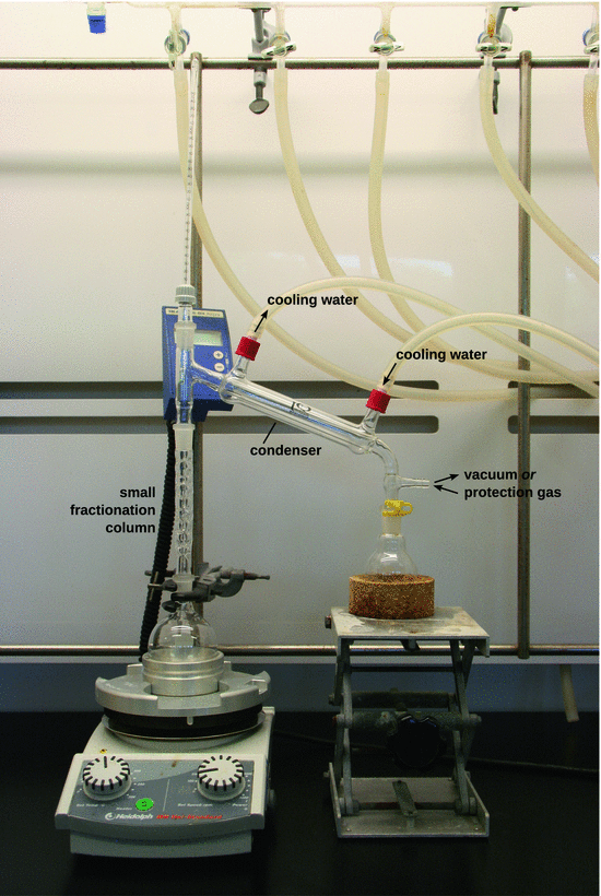
Fig. 3.19

Photograph of a distillation apparatus. For a simple distillation process as shown in Fig. 3.18, the small fractionation column is omitted

3.5.3 Fractional Distillation

In the fractional distillation, vapour is continually removed from the boiling equilibrium system, thus allowing enrichment of the more volatile component to very high purity. This is illustrated in Fig. 3.20.

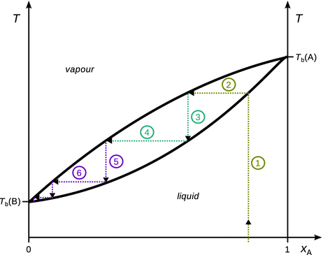
Fig. 3.20

Illustration of the fractional distillation process. Five theoretical plates (steps 2, 4, 6, 8, 10) are required to obtain pure component B from the initial mixture. For clarity, steps 7—10 are not individually labelled

✵ Step 1: A mixture of less volatile component (A; higher boiling temperature) and more volatile component (B; lower boiling temperature) is heated. The mole fraction of component B in the initial mixture is x _B ≈ 0.15.

✵ Step 2: The boiling point of the mixture at this molar composition is reached, and a vapour phase with a much higher mole fraction x _B is obtained.

✵ Step 3: The vapour from (2) condenses as it cools at a fractionation plate and reaches the boiling temperature of the liquid mixture at the new molar composition.

✵ Step 4: A new vapour phase is formed, that is further enriched in component B.

✵ Steps 5 onwards repeat this process, until an endpoint in the phase diagram is reached.

The efficiency of a fractionating column is expressed in terms of the number of theoretical plates. A theoretical plate is a hypothetical zone in which two phases establish an equilibrium with each other. This is the number of effective condensation and vapourisation steps that are required to achieve a condensate with desired composition from a given distillate. In the example in Fig. 3.20, five theoretical plates are required to obtain pure component B from the initial liquid mixture with x _B ≈ 0.15.

In distillation experiments, this process can be achieved by using Vigreux fractionation columns (Fig. 3.21) that contain spikes which form the contact devices (physical plates) between liquid and vapour and thus provide for a number of separation steps. In industrial applications, so-called bubble-cap or valve-cap trays are used. The trays are perforated, thus allowing efficient flow of vapour upwards through the column.

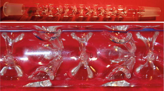
Fig. 3.21

Photograph of a Vigreux fractionation column (top) and close-up of a spike section (bottom)

The efficiency of physical plates is non-ideal and therefore the number of physical plates needed for a desired separation step is more than the calculated number of theoretical plates:

N _a is the number of actual plates, N _t the number of theoretical plates, and E is the plate efficiency. Obviously, in order to be able to calculate the number of theoretical plates for a distillation process, substantial liquid—vapour equilibrium data (i.e. phase diagrams) need to be available.

3.5.4 Mixtures of Volatile Liquids with Azeotropes

The phase diagrams of liquid mixtures we have encountered so far featured monotonous boiling and condensation curves. Some mixtures, though, show additional features in their phase diagrams. The phase diagram of the mixture illustrated in Fig. 3.22 possesses a point where boiling and condensation curves touch in one point. At this point, the liquid and vapour phases have the same composition; the point is called an azeotrope. For example, an ethanol—water mixture with 4% water forms an azeotrope that boils at 78 °C at ambient pressure.

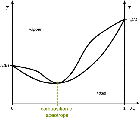
Fig. 3.22

Phase diagram of a mixture that forms a low boiling azeotrope

When boiling a liquid mixture that forms an azeotrope, evaporation will proceed without a changing composition of liquid and vapour phases. The mixture behaves as if it were a pure substance. If mixture with azeotropes are subjected to fractionated distillation, the distillation process stops being useful when the azeotrope is reached.

Two types of azeotropes can be distinguished. In low boiling azeotropes, the interactions between the two mixture components are unfavourable compared to ideal mixing. The azeotrope thus boils at the lowest temperature of all possible mixtures of the two components. An example for mixtures with low-boiling azeotropes is the ethanol—water system. In contrast, high boiling azeotropes are mixtures where the interactions between both components are more favourable when compared to the ideal case. Such azeotropes boil at the highest temperature of all possible mixtures of the two components. An example of such behaviour is a system comprising of chloroform and acetone.

3.5.5 Mixtures of Immiscible Liquids

Not all liquids can be mixed. If liquids are immiscible, then we can treat the solutions separately, but the vapour pressure of a system that comprises both components is the sum of the two vapour pressures (, ). Boiling occurs when the vapour pressure of the liquid phase equals the atmospheric pressure:

This results in an interesting consequence: When two immiscible liquids are put together, the pair of them possesses a lower boiling point than either pure liquid alone.

This behaviour is useful when heat-sensitive compounds need to be distilled. When put together with an immiscible liquid, the distillation can proceed at lower temperature than the boiling point of the pure compound. This process is typically carried out as steam distillation.

3.5.6 Phase Diagrams of Two-component Liquid/Liquid Systems

In the previous sections, we have discussed liquid mixtures that were either fully or not miscible. The mutual solubility or miscibility of two liquids is a function of temperature and composition. Of course, there are systems where the two liquid components mix under some but not all conditions. When two liquids are partially soluble in each other, two liquid phases can be observed. These are partially miscible liquids (e.g. methanol—cyclohexane, nicotine—water, phenol—water, triethylamine—water, and others). A typical phase diagram for the most common types of partially miscible liquids is shown in Fig. 3.23. The phase diagram indicates that the two liquids are fully miscible and form a one-phase liquid) at high temperatures (above T _uc), but separate into two liquid phases at lower temperatures (below T _uc). T _uc is called the upper critical temperature. The tie line is used to determine the composition of the two phases.

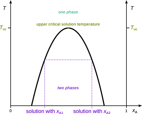
Fig. 3.23

Phase diagram for two partially miscible liquids with an upper critical solution temperature (T _uc)

There are two other cases of liquid—liquid mixtures, which are less common. The left panel in Fig. 3.24 shows the phase diagram of a mixture that possesses a lower critical solution temperature T _lc. Below this temperature, the mixture forms one liquid phase, i.e. the two components are fully miscible. Above T _lc, two liquid phases exist. This type of behaviour is observed when there are weak interactions between both components (below the critical solution temperature), such as for example in water-triethylamine.

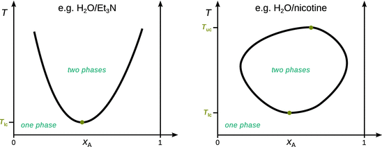
Fig. 3.24

Left: Phase diagram for mixture with a lower critical solution temperature (T _lc). Right: Phase diagram for system with both lower (T _lc) and upper (T _uc) critical solution temperatures

There also exist some systems that possess both a lower and an upper critical solution temperature, the most prominent example being water and nicotine (Fig. 3.24 right panel). These mixtures are characterised by weak interactions between both components that ensure full miscibility below the lower critical solution temperature. Above T _lc, these interactions are disrupted and there is only partial miscibility, and accordingly, two phases. Above the upper critical solution temperature, the mixture is homogenised and exists as a single liquid phase.

3.5.7 Phase Diagrams of Two Component Liquid—Vapour Systems

If we now consider a mixture of two partially miscible liquids and also form a low-boiling azeotrope, we arrive at a fairly common behaviour of real substances. Both properties, partial miscibility and azeotrope formation, emphasise the fact that the molecules of the two components tend to avoid each other.

This behaviour is possible with two different options:

✵ the liquids may become fully miscible before they boil, i.e. the azeotrope is well separated from the upper critical solution temperature (Fig. 3.25 left), or

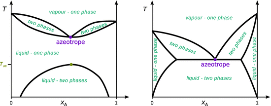
Fig. 3.25

Phase diagrams of two-component liquid—vapour systems of partially miscible liquids with a low-boiling azeotrope. Left: The liquids fully mix before the mixture starts to boil. Right: The mixture starts to boil before the two components become fully miscible

✵ boiling occurs before the two liquids are fully mixed, i.e. the azeotrope and the upper critical solution temperature merge (Fig. 3.25 right).

3.5.8 Phase Diagrams of Two-component Solid—Liquid Systems

In the previous sections, we considered systems consisting of two components and discussed their liquid and vapour phase behaviour. In the same fashion, solid and liquid phases can be characterised. Conceptually, there is no difference in the way such phase diagrams are interpreted. As an example, Fig. 3.26 illustrates the phase diagram of two partially miscible solids whose melting point occurs before the two solids are fully mixed.

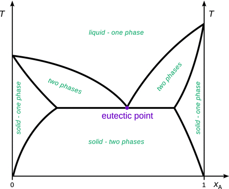
Fig. 3.26

Phase diagram of two partially miscible solids. The mixture with the lowest melting point has eutectic composition

It is immediately obvious that this phase diagram is highly similar to the one we have seen before (Fig. 3.25 right) in the case of a two-component liquid—vapour system where the two liquids were partially miscible and boiling occurred before full mixing of the liquids. For solids, the mixture with the lowest melting point is called the eutectic point (as opposed to the azeotrope in the liquid—vapour systems).

3.5.9 Phase Diagrams of Three-component Systems

Of course, mixtures can be made of more than just two components, but visualisation of phase diagrams for higher order systems becomes challenging. For three-component systems, it is still possible to plot two-dimensional phase diagrams. Instead of a Cartesian x—y diagram, a triangular coordinate system can be used, that allows to plot the composition of each of the three components (A, B, C) in the system. However, such phase diagrams are restricted to a particular temperature and pressure.

Like for binary systems before, we can state that the sum of the individual mole fractions is 1:

Figure 3.27 illustrates such a triangular phase diagram, showing the mole fractions for a ternary system, at a certain pressure and temperature. The phase separation of the water-butanol-acetic acid system is shown with the grid of the coloured coordinate system in the background.

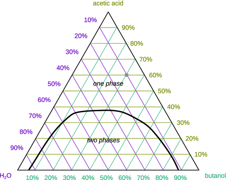
Fig. 3.27

Qualitative ternary phase diagram for the three liquids water, acetic acid and butanol. The one and two phase regions of this system are separated by the black line. The arbitrary point marked in the diagram represents 10% water, 60% acetic acid and 30% butanol

3.5.10 Cooling Curves

Cooling curves show how the temperature in a system changes during the time course of the cooling process. Pure liquid, solid or gas phases have smooth, monotonous changes in temperature, until the process approaches a phase transition.

The phase transitions of pure substances proceed along the pathway of gas → liquid → solid, occur at single temperatures and are exothermic (they are endothermic along the opposite pathway). During the phase transition, the temperature does not change until the phase of the substance has been fully converted. This is illustrated in Fig. 3.28 for a phase diagram with three (left panel) and two phases (middle panel).

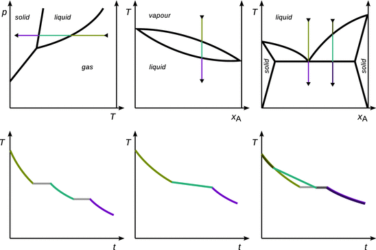
Fig. 3.28

Cooling processes of a pure substance with three phases (left), a pure substance with two phases (middle), and a binary solid—liquid mixture with eutectic point. The upper row shows the phase diagrams, and the lower row the cooling curves as time-temperature diagrams

Phase transitions during cooling of mixtures also proceed along the pathway of gas → liquid → solid, but occur over a temperature range (see Fig. 3.28 right panel). As with pure substances, the phase transitions during cooling of mixtures are exothermic processes. Therefore, the temperature during these transitions is not constant, but abrupt changes in the overall cooling curve are still visible when the cooling process begins and ends (i.e. the phase transition still leads to occurrence of kinks in the graph). Notably, azeotropes and eutectics behave like a pure substance and show a constant temperature during the phase transition.