Physical Chemistry Essentials - Hofmann A. 2018
Solutions of Electrolytes
4.3 Electrolytes in Solution
4.3.1 Solubility Product
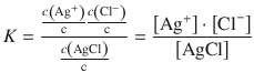
In the previous section, we have introduced the silver/silver chloride electrode as a frequently used reference electrode. The electrode is made of a silver wire coated with silver chloride that is immersed into a solution containing chloride ions. The step which determines the potential of this electrode (half-cell) is the transition of Ag+ ions from the electrode into solution. Here, the metal ions (Ag+ (s)) are in a heterogeneous equilibrium between the solid electrode material (AgCl(s)) and the dissolved ions (Ag+ (aq), Cl− (aq)). A saturated aqueous AgCl solution contains only 13 μM Ag+ and 13 μM Cl− ions; the equilibrium of the following disassociation reaction is thus on the left hand side
![]()
and results in an equilibrium constant of small value:
(4.31)
Remember that H2O is omitted from calculation of the equilibrium constant, since it is neither consumed nor produced. The concentration of any solid substances are considered to be constant in solvation reactions, hence c(AgCl) = const.
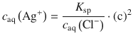
The silver chloride concentration can thus be multiplied into the equilibrium constant, yielding a new constant, the solubility product, which is solely a function of the concentration of dissolved ions:
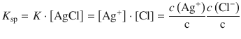
(4.32)
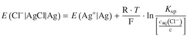
The electrode (half-cell) potentials are themselves potential differences (see Fig. 4.9). They arise from the transition of ions from the solid to the dissolved state. To stay consistent with the nomenclature used in previous sections, we will denote these differences as E and E —, respectively, to indicate that we are referring to an electrochemical half-cell. In analogy to the way in which we derived Eq. 4.27, we can formulate an expression for the potentials arising from Ag+ transitions in the silver/silver chloride electrode, by using Eq. 4.32:
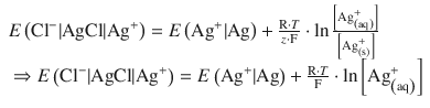
(4.33)
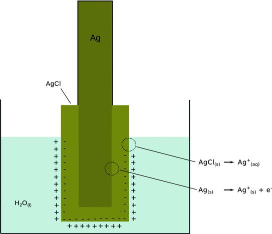
Fig. 4.9
Illustration of transition processes at electrodes and the generation of an electrode potential. Positively charged ions transition from the solid to the dissolved state. This changes the electroneutrality and leads to generation of an electrostatic double layer. The double layer is responsible for the electrode potential
From Eq. 4.32 we obtain
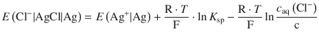
which we can substitute into Eq. 4.33:
(4.34)
Using the logarithm rule of ![]() we obtain:
we obtain:
As ![]() is a constant, it can be combined with the standard potential of the Ag+ | Ag transition:
is a constant, it can be combined with the standard potential of the Ag+ | Ag transition:
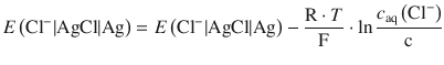
(4.35)
Determining the Solubility Product from Standard Electrode Potentials
Since the solubility product of a poorly soluble salt forms part of the standard electrode potential if that salt is part of the solid electrode material, one can determine the solubility product from these (tabulated) standard electrode potentials. Comparison of Eqs. 4.34 and 4.35 shows that the right hand sides of both equations can be set equal:
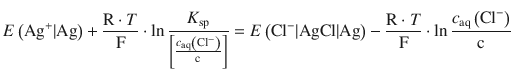
Using the logarithm rule of ln ![]() , we obtain:
, we obtain:
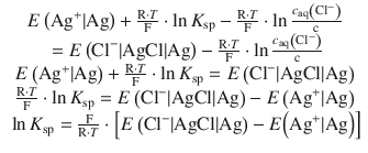
(4.36)
The tabulated standard electrode potentials for the two reactions are:
![]()
![]()
This yields for Eq. 4.36:
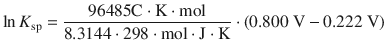
With 1 C = 1 J V−1 this resolves to:
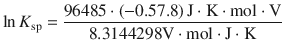
![]()
![]()
From Eq. 4.32, we know that the units of the solubility product for silver chloride are:
![]()
and therefore:
![]()
4.3.2 Colligative Properties and the van’t Hoff factor
As we have seen in Sect. 3.2.2, colligative properties result from the reduction of the chemical potential μ∗ solvent of the pure liquid solvent, as a result of the presence of the solute. For an ideal solvent/solution we can state:
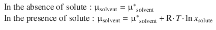
(3.13)
Because x solute is the mole fraction, its value in case of a solution is larger than 0 and less than 1:
![]()
Hence the second term in Eq. 3.13 is always negative and thus μsolvent < μ∗ solvent.
These properties depend on the particular solvent and on the concentration of solute, but not on the nature of the solute. If we assume ideal solutions, then the solute and the solvent have identical intermolecular forces. Therefore, the enthalpy of solution is zero (ΔH sol = 0), since the potential energy of solvent and solute molecules is not affected. However, the intermixing of solute and solvent will raise the entropy of the solution: ΔS sol > 0. Therefore, the lowering of the chemical potential of the liquid solvent is an entropic effect.
In summary, colligative properties:
✵ Do not depend on the chemical nature of the solute
✵ Depend on the concentration of the solute
✵ Depend on the nature of the solvent
✵ Are entropic effects, thus depend on the number of dissolved particles.
There are four important colligative properties (see Table 4.4), all of which are related to the concentration of the solute.
Table 4.4
Colligative properties
|
Effect |
Equation |
Parameters |
Concentration |
Lowering of vapour pressure ( Raoult’s law) |
p = x · p ∗(3.12) |
p ∗: vapour pressure of pure liquid |
Mole fraction x |
Melting point depression |
ΔT f = K f · b(4.37) |
K f: cryoscopic constant |
Molality b |
Boiling point elevation |
ΔT b = K b · b(4.38) |
K b: ebullioscopic constant |
Molality b |
Osmosis |
Π = c · R · T(4.39) |
Π: osmotic pressure |
Molar concentration c |
For historical reasons, different types of concentrations are used for the different phenomena (Table 4.5). The concentrations are:
Table 4.5
Commonly used measures of concentration
Mole fraction |
|
[x] = 1 |
(2.74) |
Molality |
|
[b] = 1 mol kg−1 |
(4.40) |
Molar concentration |
|
[c] = 1 mol l−1 |
(2.73) |
Mass ratio |
|
[w] = 1 |
(4.41) |
Raoult’s law, which describes the lowering of the vapour pressure of a liquid in the presence of solutes has already been described in an earlier Sect. 3.2.1. Intriguingly, the fact that the vapour pressure of a solution is lower than that of the pure solvent results in the observation that the boiling point of a solution is higher than that of the pure solvent.
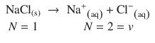
In order to consider the entropic effects of solutes, a factor that considers the number of dissolved particles in the solution needs to be introduced. This is especially important for electrolytes, as the number N of particles always increases upon dissociation:
Therefore, the van’t Hoff equation for the osmotic pressure is corrected by a factor i, called the van’t Hoff factor:
![]()
(4.39)
Similarly, for boiling point elevation and melting point depression one obtains:
![]()
(4.38)
![]()
(4.37)
For an ideal (i.e. infinite) dilution, the van’t Hoff correction factor i approaches the theoretical number of ions v into which the solute molecule dissociates (see Fig. 4.10). The variation of the van’t Hoff factor from the theoretically expected dissociation numbers for both electrolytes and non-electrolytes may arise from the following phenomena:
✵ Difference in internal pressure of solute and solvent
✵ Polarity
✵ Compound formation or complexation
✵ Association of either solute or solvent
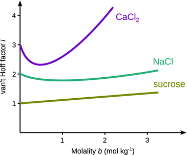
Fig. 4.10
The van’t Hoff factor i approaches the theoretical number of ions into which an electrolyte dissociates (ν) only at infinite dilution. For non-electrolytes, the van’t Hoff factor may also differ from the theoretical value of ν = 1 at increasing concentrations
In case of electrolytes, additional effects arise from:
✵ The dissociation of weak/strong electrolytes
✵ Interaction of the ions of strong electrolytes.
4.3.3 Degree of Dissociation
If the deviation of the van’t Hoff factor i from the theoretically expected value v is due to dissociation only, then the degree of dissociation α can be determined as per:

(4.42)
where v is the theoretical number of ions yielded per solute molecule (e.g. for CaCl2: v = 3).
The degree of dissociation α can be reliably estimated for weak electrolytes, as there are only few ions at all concentrations, and therefore other solution effects are negligible.
For strong electrolytes, Eq. 4.42 works well at low concentrations, but substantially deviates from experimental observations at moderate or strong concentrations, due to interactions between ions. With increasing concentrations, attractive interactions between dissolved electrolytes become important, and ion pairs or triplets may form (Fig. 4.11). Since ions involved in those pairings no longer account as individual ions, the degree of dissociation is less than expected.
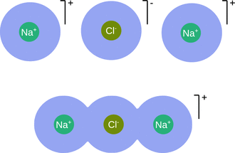
Fig. 4.11
Illustration of ion association. In solution, ions of opposite electrical charge may come together to form a distinct chemical entity. Top panel: fully solvated ions; bottom panel: an ion triplet with solvent sharing
4.3.4 Activities and Ionic Strength
In cases such as the one described in the previous section, where significant deviations from the ideal behaviour need to be considered, it is appropriate to use an ’effective concentration’. Therefore, for strong electrolytes as well as weak electrolytes in the presence of salts (e.g. buffer systems), activities instead of concentrations should be used in order to quantify the deviation from the completed dissociation behaviour.
We have previously defined the activity a such that the following equation is true for a real liquid (see Sect. 3.2.3):
![]()
(3.12)
where the activity a (non-ideal solution) is related to the mole fraction x (ideal solution) by a scaling factor called the activity coefficient γ:
![]()
(3.13)
Importantly, activity can be defined in terms of any other concentration measure (see Table 4.6). The activity of solutes is usually less than the concentration, but it approaches the same value as the concentration at high dilution. Activities may be different for cations and anions of an electrolyte. For ideal solvents, the activity coefficient γ = 1, for non-ideal solvents, the activity coefficient approaches 1 at very high concentration of the solvent.
Table 4.6
Definition of activity in terms of frequently used concentration measures
Activity in terms of the mole fraction x |
a = γ x ⋅ x |
(4.43) |
Activity for a volatile solvent (Raoult’s law: p = x ⋅ p ∗) |
|
(4.44) |
Activity in terms of molality b |
a = γ b ⋅ b |
(4.45) |
Activity in terms of molar concentration c |
a = γ c ⋅ c |
(4.46) |
When comparing activities of electrolytes, experimental conditions should be chosen to ensure constant ionic strength. If a solution contains N different types of ions with the charge states z 1 , z 2 , …, z N and at concentrations c 1 , c 2 , …, c N , it is appropriate to use an average concentration. The ionic strength I is such an averaged concentration, weighted by the square of the charge state:
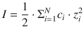
(4.47)
Here, c i is the molar concentration and z i is the charge of the ith ion; N is the number of different ions in the solution.
The ionic strength is important in many biochemical applications. For instance, when evaluating the effect of pH on an enzymatic reaction, the effect of the salt concentration in the buffer may obscure the results, unless the buffer is adjusted to ionic strength in each experiment.
4.3.5 pH Buffers
In analogy to the solubility product of electrolytes (see Sect. 4.3.1), one can consider the following dissociation of water
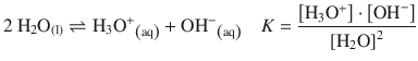
(4.48)
and define the ion product of water as
![]()
(4.49)
The equilibrium constant K has a very small numerical value, since the equilibrium of reaction 4.48 resides on the left hand side. Since the molar concentration of water can be assumed constant (c = 55.56 mol l−1), it is combined with the equilibrium constant K to yield the ion product of water: K w = 1.0 · 10−14.
Since in pure water, the amounts of hydronium (H3O+) and hydroxide (OH−) ions resulting from the dissociation reaction above are equal, the concentration of hydronium ions (for convenience frequently replaced by protons) can be calculated from Eq. 4.49:
![]()
(4.50)
This gives rise to the definition of the pH and pOH, which are calculated as the negative decadic logarithms of the H+ and OH− concentrations, respectively:
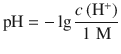
(4.51)
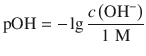
(4.52)
From Eq. 4.50 follows that:
![]()
(4.53)
The pH of aqueous solutions can be affected by:
✵ Neutral salts, which may modify the ionic strength
✵ Water addition, which may either change activity coefficients or act as a weak acid or base
✵ Temperature, which changes K w and K a or K b in case of acids/bases (see below).
Therefore, pH buffers are of high practical importance in many (bio-)chemical formulations (e.g. drug preparations, creams, etc) as well as living cells where, for example, buffers in blood keep the pH at ~7.4 (blood pH outside the range 6.9 and 7.8 puts life in danger).
Buffers are compounds or mixtures of compounds that withstand a change in pH upon addition/generation of acid or base (in a reasonable window). Buffer compounds are typically weak acids with their conjugate bases, or weak bases and their conjugate acids. For example, on addition of a strong acid to a solution containing equal quantities of acetic acid and sodium acetate, the hydrogen ions react with the acetate according to
![]()
thus converting the hydronium ion to water and eliminating the acidic property.
Obviously, the capacity of the buffer system to ’eliminate’ additional hydronium ions will be exhausted, when all available molecules of the weak base have been consumed. The amount of either strong acid or base that can be added before a significant change in the pH will occur is a matter of stoichiometry. The maximum amount of strong acid that can be buffered is equal to the amount of conjugate base present in the buffer. Similarly, the maximum amount of base that can be tolerated is equal to the amount of weak acid present in the buffer.
The pH of a solution that contains a buffer system consisting of a weak acid and conjugate base can be calculated based on the equilibrium of the dissociation reaction
![]()
where HA denotes the acid (e.g. H3CCOOH) and A− the conjugate base (e.g. H3CCOO−). The equilibrium constant K a for the dissociation reaction is given by:
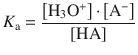
This yields for the concentration of hydronium ions:
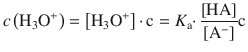
We divide the left and right hand side of this equation by the unit of the molar concentration (1 M), and then subject both sides to a logarithmic operation, with lg = log10:
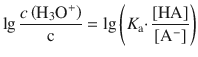
Using the logarithm rule of log(a ⋅ b) = log a + log b, we obtain:
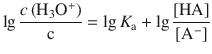
After multiplying the equation with (−1):
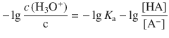
we recognise that the left hand side is the definition of the pH: ![]() and the expression
and the expression ![]() defines the pK a of the acid HA:
defines the pK a of the acid HA: ![]()
This yields:
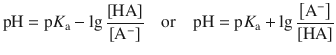
(4.54)
which is known as the Henderson-Hasselbalch equation.
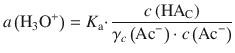
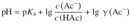
For real (non-ideal) situations, the equilibrium constant needs to be set up with activities instead of concentrations. If we consider a buffer system consisting of acetic acid (HAc) and acetate (Ac−) for illustration, this yields:
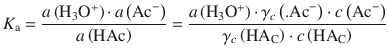
Since HAc constitutes the solvent, and is thus present at a large concentration (i.e. its mole fraction approaches 1), we know from Sect. 4.3.4 that:
γx → 1 as x → 1, therefore γc(HAc) ≈ 1, which yields:
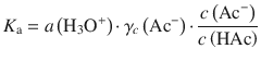
Resolving for a(H3O+) yields:
In order to the logarithm of both sides, we need to divide by the units of activity which in this case are 1 M:
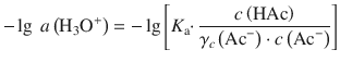
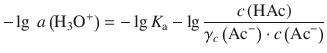
Using the logarithm rule log(a ⋅ b) = log a + log b, we obtain:
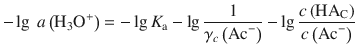
With the rule ![]() , this yields:
, this yields:
and therefore:
(4.55)
which is the Henderson-Hasselbalch equation considering activities. Comparison with Eq. 4.54 shows that the additional term of lg γ(Ac−) needs to be taken into account.
4.3.6 Applications of Conductivity Measurements
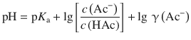
When titrating weak acids (bases) with strong bases (acids), the determination of the end point of titration may be difficult due to the buffering properties described in the previous section. In such cases, conductivity measurements (also called conductometry) can be used to detect the end points of titrations. Conductometric titrations are also a useful alternative for acid-base titrations where indicators can not be used, because the sample or titrant are coloured. The observable parameter in these titrations is the conductivity κ (see Eq. 4.10).
Figure 4.12 compares observations in conductometric titrations with different acid/base pairings. When a strong base (e.g. NaOH, the analyte) is titrated with a strong acid (e.g. HCl, the titrant), the solution initially contains Na+ (aq) and OH− (aq) ions, therefore high conductivity is observed (Fig. 4.12, left panel). As the titration proceeds, the conductivity falls sharply since OH− (aq) ions react with H+ (aq) to neutral H2O and the added Cl− (aq) ions replacing OH− (aq) have a lower conductivity than OH− (aq) (see Table 5.5). At the end point, the exact amount of H+ (aq) has been added to match the amount of OH− (aq), and the solution shows a conductivity expected of a solution of NaCl in water. As more titrant is added, the conductivity begins to rise sharply, due to H+ (aq) having higher conductivity than Na+ (aq). Determination of the end point is conveniently done by extrapolating the two branches of the conductometric plot.
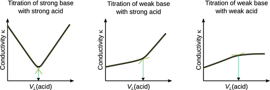
Fig. 4.12
Schematic plots of conductometric titration data for strong acid/strong base (left), strong acid/weak base (middle), weak acid/weak base (right). Typical experimental conductivity values for such titrations are in the range of μS cm−1
When a weak base (e.g. NaAc) is titrated with a strong acid (e.g. HCl), the initial conductivity of the solution is low, since the salt of the weak base is only partially dissociated (Fig. 4.12, middle panel). Addition of H+ (aq) and Cl− (aq) leads to a rise in conductivity, as the acid-base reaction causes dissociation of the salt and thus releases Na+ (aq). After the amount of base is been matched by H+ (aq) at the endpoint, the conductivity rises sharply, as now excess H+ (aq) become available which possess substantially higher conductivity than any other ions (see Table 5.5).
4.3.7 The Debye-Hückel Theory
So far, any deviation from ideal behaviour has been treated by an empirical approach. In order to be able to account for non-ideal behaviour, the concentration of an electrolyte has been replaced with the activity, and we demanded that all underlying thermodynamic relations such as the variation of the chemical potential (Eq. 3.12) should then remain valid even for non-ideal solutions. The value of the activity may be found by experimentally determining the activity coefficient and using the known concentration. With these activity values, fundamental thermodynamic quantities such as the chemical potential can then be calculated.
Experimental Determination of Activity Coefficients
The activity a and the activity coefficient γ are intimately linked to the mole fraction or concentration whenever a system deviates from ideal behaviour (see Table 4.6). Any such phenomena can thus be used, in principle, to determine activity coefficients.
For example, the colligative property of vapour pressure lowering by a solute may be used to determine the activity coefficient of the solvent. From Raoult’s law, we know that
![]()
(3.12)
where x is the mole fraction of the solute, p the vapour pressure of the solution and p * the vapour pressure of the pure solvent. In Table 4.6, we have thus defined the activity of a non-ideal solvent as
![]()
(4.44)
Remembering that the activity in terms of the mole fraction is generally defined as
![]()
(4.43)
we obtain:
![]()
(4.56)
which allows for the experimental determination of the activity coefficient γ of the solvent directly from observation of the colligative property of vapour pressure lowering by a solute. The only requirement is that the vapour of the solution/solute behaves as an ideal gas. If that is not the case under the chosen conditions, fugacities instead of pressures need to be used.
Debye and Hückel developed a theoretical basis to quantify the non-ideal behaviour of electrolyte solutions. Their theory is based on the following assumptions:
✵ The electrolyte solution needs to be dilute (i.e. c < 0.01 mol l−1)
✵ The electrolytes are completely dissociated into ions
✵ On average, each ion is surrounded by ions of opposite charge (see Fig. 4.13).
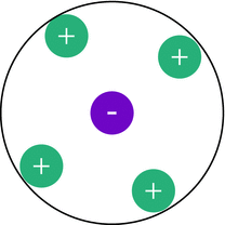
Fig. 4.13
The Debye-Hückel theory assumes an ionic atmosphere: on average, each ion is surrounded by a sphere of counter-ions
Based on these assumptions, Debye and Hückel calculated the chemical potential of a completely dissociated electrolyte from the chemical potentials of the cat- and anions. These calculations result in a relationship between the mean activity coefficient γ± and the ionic strength I of the solution, called the Debye-Hückel limiting law:
![]()
(4.57)
where z + and z − are the charge numbers of the cat- and anion of the electrolyte, and I is the ionic strength as defined in Eq. 4.47. A is a constant for the solvent of interest; in case of aqueous solutions at θ = 25 °C, A = 0.5099 dm3/2 mol−1/2.
Due to the principle of electroneutrality (see Sect. 4.1.2), one can only prepare solutions that contain cat- as well as anions. Therefore, the Debye-Hückel theory provides the above relationship only for a mean activity coefficient. Notably, electrolytes that possess the same charge numbers also possess the same mean activity coefficients.
Using the Debye-Hückel limiting law, we can now return to the Henderson-Hasselbalch equation for the non-ideal solutions, illustrated by the acetic acid/acetate buffer system (Eq. 4.55):
(4.55)
The last term in this equation can be evaluated from Eq. 4.57 as follows:
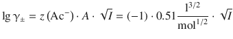
Therefore:
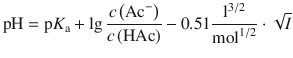
(4.58)
4.3.8 Tonicity
As well as controlling the pH of a solution, it is often necessary to control the osmotic pressure Π of a solution, especially when preparing biochemical buffers. For example, in cases where membranes are involved, a difference in the osmotic pressure between the two sides of the membrane may have devastating effects and cause swelling, contraction or even rupture of the membrane.
The measure of the osmotic pressure gradient of two solutions that are separated by a semi-permeable membrane is called tonicity. It is thus a qualitative description of the relative concentrations of solutes in the two solutions and determines the direction of diffusion. Three different cases can be distinguished: hypertonic, hypotonic and isotonic solutions. Commonly, tonicity refers to the osmotic pressure, but it can also be defined for any other colligative property (melting point, boiling point). Isotonic solutions thus describe solutions that possess the same colligative properties.
In biological settings, a hypertonic solution is one with a higher concentration of solutes outside the cell than inside the cell. Therefore, hypertonic solutions will cause diffusion of water out of the cell in order to balance the concentration of the solutes. Hypotonic solutions, in contrast, possess a lower concentration of solutes outside the cell than is found inside the cell. The direction of diffusion in this case is thus such that water flows into the cell, causing swelling and possible bursting. If an outside solution provides the same concentration of solutes as found inside the cell, then this solution is called isotonic. Water molecules diffuse through the membrane in both directions at equal rates. Isotonic solutions have great importance for biochemical and medical applications; they are for example used as intravenously infused fluids with patients or as washing solutions for the eye in laboratories.
The Concentration of an Isotonic NaCl Solution
The melting point of human blood and tears is −0.52 °C. Determine the mass ratio w of an isotonic NaCl solution in water (K f = 1.86 K kg mol−1).
The colligative property of melting point depression is given by:
![]()
(4.37)
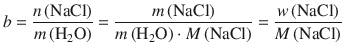
The molality b is given by:
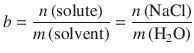
(4.40)
The concentration of solute is expressed here as the mass ratio w, which is defined as:
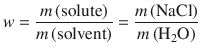
(4.41)
We thus obtain from Eq. 4.40:
This yields for the mass ratio w:
![]()
From Eq. 4.37, we can substitute for the molality:
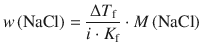
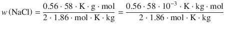
![]()