Physical Chemistry Essentials - Hofmann A. 2018
Molecules in Motion
5.1 Transport Processes
We have already seen that physico-chemical processes do not always require a chemical reaction to proceed, such as for example when considering solutions or phase changes. Irreversible processes that arise from non-equilibrium conditions may also include the spatial translocation of objects and properties. In particular, one can observe the transfer of
✵ matter
✵ energy
✵ any other property.
Such transport processes are fundamental processes in biological settings (molecular transport in the cell) and engineering (e.g. liquid flow, thermo devices, etc). Four important instances of transport processes are:
✵ diffusion: migration of matter along a concentration gradient
✵ thermal conduction: migration of energy along a temperature gradient
✵ electric conduction: migration of charges along an electric potential gradient
✵ viscosity: migration of a linear momentum along a velocity gradient.
We have already considered electric conduction in Sect. 4.1, and will consider these properties again in more detail in Sects. 5.1.4—5.1.6. However, to introduce some fundamental concepts and parameters, we shall start with an introduction to the kinetic molecular theory of gases.
5.1.1 The Kinetic Molecular Theory of Gases
In the kinetic molecular theory of gases, we only consider energy contributions that arise from the kinetic energy of the individual gas molecules. We assume an ideal gas, and therefore contend that
✵ the gas consists of molecules of mass m in random motion
✵ the molecules have negligible size
✵ the molecules interact only through brief, infrequent, elastic collisions.
Elastic collisions are those where the total translational kinetic energy of molecules is conserved.
From this kinetic molecular theory, one can derive an equation that relates pressure and volume of an ideal gas with the speed of the individual gas molecules:
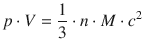
(5.1)
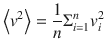
with c being the root mean square speed of the molecules, i.e. a speed averaged over the entire population of gas molecules:

(5.2)
In the above equation, ⟨v 2⟩ is the arithmetic mean of the squared speeds:
The speed of the individual gas molecules only depends on the temperature (see Eq. 2.1 which defines the relationship between temperature and average kinetic energy of molecules). Therefore, at constant temperature, the root mean square speed c will also be constant. It follows straight from Eq. 5.1 that at constant root mean square speed c (i.e. constant temperature) the product p·V is constant. This is otherwise known as Boyle’s law, which states that
the absolute pressure exerted by a given mass of an ideal gas is inversely proportional to the volume it occupies, if the temperature and amount of gas remain unchanged within a closed system:
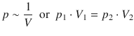
(5.3)
Since we are considering an ideal gas, we can further develop Eq. 5.1:
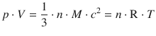
(5.4)
and derive an expression for the root mean square speed of the gas molecules:
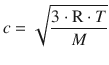
(5.5)
Analysis of Eq. 5.5 shows that
✵ the higher the temperature, the higher the speed of the molecules, and
✵ heavy molecules travel slower than light molecules.
5.1.2 The Maxwell—Boltzmann Distribution
The root mean square speed c of the gas molecules is an averaged speed over the entire population of gas molecules in the system. Obviously, the speeds of individual gas molecules vary and span a range of different values. A molecule may be travelling rapidly, but then collide and travel slower. It may then accelerate again, only to be slowed down by the next collision.
The distribution of speeds (velocities) can be calculated based on the Boltzmann distribution, which is a probability distribution over various possible states of a system frequently used in statistical mechanics (Maxwell 1860a, 1860b). The resulting function is called the Maxwell—Boltzmann distribution:
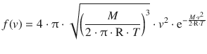
(5.6)
In Eq. 5.6, the exponential factor ![]() resembles the well-known Boltzmann factor that describes the ratio of two states which only depends on the energy difference between the two states:
resembles the well-known Boltzmann factor that describes the ratio of two states which only depends on the energy difference between the two states:
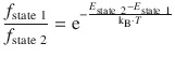
(5.7)
A graphical representation of the Maxwell—Boltzmann distribution for either varying molecular masses or temperatures is shown in Fig. 5.1. For a particular gas (Fig. 5.1 right panel, molecular mass is constant), the average speed of the molecules, as indicated by the position of the peak, increases with increasing temperature. At the same time, the distribution of different speeds becomes lees uniform within the population of gas molecules when the temperature increases; this is obvious from the distribution curves spreading out. Notably, the areas underneath the curves remain the same, since the number of gas molecules in the system is considered to be constant.
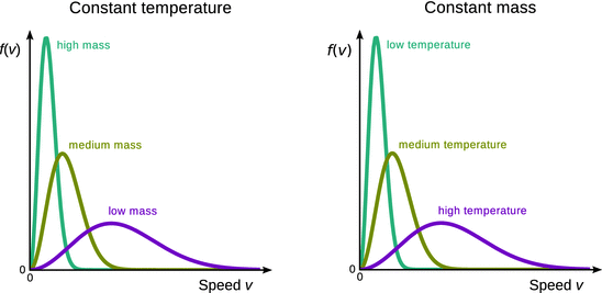
Fig. 5.1
Graphical representation of the Maxwell—Boltzmann distribution (Eq. 5.6) for either varying temperatures or molecular masses
When comparing different gases with different molecular masses (Fig. 5.1 left panel) at the same temperature (and assuming the same number of molecules), the Maxwell—Boltzmann distribution shows that lighter molecules possess higher average speeds than heavier molecules. Also, the distribution of individual speeds is less uniform in populations of lighter molecules.
5.1.3 Transport Properties
The generally accessible concept of flux as a stream of moving bodies (objects that have a mass) can be readily expanded to any object, including those that have no mass, such as physical properties. The migration of a property, i.e. property transport, can phenomenologically be described by its flux:
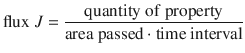
(5.8)
In order to calculate the total quantity of a property that is migrating, one can re-arrange above equation to obtain:
![]()
In general, we can distinguish two types of properties migrating, matter and energy (Table 5.1):
Table 5.1
Migration of properties
|
Property migrating |
Process |
Flux |
Units of flux |
Matter |
Diffusion |
Number of molecules per area per time |
|
Energy |
Thermal conduction |
Energy per area per time = power per area |
|
Momentum |
Laminar flow |
Force per area |
|
5.1.4 Diffusion: Flux of Matter
In most cases, it is found that the flux J of one property is proportional to the first derivative of another. This fundamental observation is called the general transport equation.
For example, the flux of molecules (property 1 = matter) that migrate by diffusion along a particular direction x is proportional to the first derivative of the concentration of these molecules (property 2 = concentration) along that direction. If we choose to work with the molar concentration c, then the first derivative of c with respect to the travel coordinate x is ![]() , and we can denote the above rule mathematically as:
, and we can denote the above rule mathematically as:

(5.9)
This relationship is known as Fick’s first law of diffusion.
Since matter migrates from areas of high concentration to low concentration, the direction of migration is opposite to the concentration gradient. The opposite direction between flux and concentration gradient is expressed by a minus sign, when the proportionality relationship in Eq. 5.9 is converted to an equation:
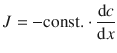
In this equation, the constant factor will become D′, a coefficient for the diffusion process:

(5.10)
Practically, it is not the molar concentration c that is used for the particle flux, but rather the concentration expressed as number of particles per volume, ![]() . Therefore, Eq. 5.10 is transformed as per:
. Therefore, Eq. 5.10 is transformed as per:
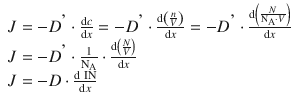
(5.11)
Equation 5.11 contains the diffusion coefficient D that is commonly used. (According to the above transformations, D and D′ are related as per ![]() ). The SI units of the different components in eq. 5.11 are given in Table 5.2.
). The SI units of the different components in eq. 5.11 are given in Table 5.2.
Table 5.2
Units of the parameters for particle flux (diffusion)
|
Parameter |
Units |
Explanation |
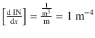
Concentration gradient |
|
Number of molecules per volume travelling over a distance |
Flux |
[J] = 1 m−2 s−1 |
Number of molecules passing an area per time interval |
Diffusion coefficient |
[D] = 1 m2 s−1 |
5.1.5 Thermal Conduction: Flux of Energy
Energy migrates along a temperature gradient; this transport is called thermal conduction. Similar to the diffusion process, energy migrates from high to low temperature, i.e. opposite the temperature gradient. When applying the general transport equation for thermal conduction, we therefore need to include a minus sign to account for the opposite direction of flux and gradient:

(5.12)
The proportionality constant κ is called the thermal conductivity. The SI units of the different components in Eq. 5.12 are given in Table 5.3.
Table 5.3
Units of the parameters for thermal conduction
|
Parameter |
Units |
Comment |
Temperature gradient |
|
|
Flux |
[J] = 1Jm−2s−1 = 1Wm−2 |
Also called the heat flux density |
Thermal conductivity |
[κ] = 1JK−1m−1s−1 = 1WK−1m−1 |
5.1.6 Viscosity: Flux of Momentum
A substance streaming through a tube (Fig. 5.2) can be considered as consisting of laminar layers that flow in the same direction. If the substance is very fluid (’non-viscous’) and flows through the tube with negligible resistance, then all layers move with the same speed. In contrast, the speed of the individual layers in a viscous substance are different: at the walls, the liquid moves with a substantially lesser speed than in the centre of the tube, giving rise to a ’U’- or ’V’-shaped profile.
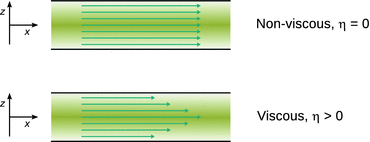
Fig. 5.2
Top: If a substance flow in a tube has negligible resistance, the speed is the same all across the tube. Bottom: When a viscous substance flows through a tube, its speed at the walls is substantially less than in the centre of the tube
When molecules from an outer layer (which moves at slow speed) switch to a neighbouring layer that moves faster, the neighbouring layer will be retarded because of the lower momentum of the switching molecules. The opposite will happen when molecules switch from a faster (inner) to a slower moving (outer) layer.
When molecules switch from one layer to another (a movement perpendicular to the flow direction z), then a momentum of (m·v x ) or (m·v y ) migrates from one layer to another. The flux of momentum is described by:
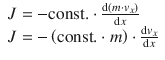
(5.13)

(5.14)
The constant of proportionality, η, is called the viscosity. If all layers move at the same velocity, the gradient ![]() is zero, and there is no flux of momentum; the substance may still have a viscosity, though! The SI units of the different components in Eq. 5.14 are given in Table 5.4.
is zero, and there is no flux of momentum; the substance may still have a viscosity, though! The SI units of the different components in Eq. 5.14 are given in Table 5.4.
Table 5.4
Units of the parameters for the momentum flux
|
Parameter |
Units |
Comment |
Momentum gradient |
|
|
Flux |
[J] = 1 kg m−1s−2 = 1 N m−2 |
|
Viscosity |
[η] = 1 kg m−1s−1 = 1 N s m−2 = 10 P |
The unit poise is named after Jean Léonard Marie Poiseuille |
When discussing the flow of a substance through a tube in the above paragraph, most likely liquids came to mind; for example, water as a liquid with negligible viscosity, and glycerol as a liquid with considerable viscosity. However, these phenomena are not limited to liquids. For example, the shape of the Bunsen burner flame is due to the velocity profile across the tube.
5.1.7 The Transport Parameters of the Ideal Gas
Earlier in this section, we introduced the kinetic molecular theory of gases (Sect. 5.1.1), and started to link the behaviour of particular gas molecules to macroscopic laws. We then learned about transport properties and can now apply these to an ideal gas. Using the kinetic theory, expressions for the different transport parameters can be derived. We will not derive these relationships rigorously, but rather discuss their impact on the gas molecules.
The diffusion coefficient D of the ideal gas is obtained as per

(5.15)
Here, λ is the mean free path length, i.e. the average distance a molecule travels without collision; c is the mean speed of the molecules.
We can predict the following effects:
✵ Since the mean free path λ of gas molecules decreases with increasing pressure (more collisions), Eq. 5.15 tells us that the diffusion coefficient D also decreases with increasing pressure. This means that at higher pressure, molecules diffuse more slowly.
✵ The mean speed c increases with increasing temperature, and according to Eq. 5.15 so does the diffusion coefficient D. This means that at higher temperatures, molecules diffuse more quickly.
✵ The mean free path λ (and thus the diffusion coefficient D) increases when the collision cross-section of molecules decrease. Smaller molecules therefore diffuse quicker than large molecules.
The thermal conductivity κ of an ideal gas A is given by
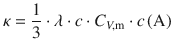
(5.16)
where λ and c are the mean free path and mean speed as before. C V,m is the molar heat capacity at constant volume and c(A) the molar concentration of the gas.
This allows the following predictions:
✵ The mean free path λ is inversely proportional to the concentration (high concentration means more molecules which make the occurrence of collisions more likely, thus decreasing the mean free path). The thermal conductivity κ would thus be expected to decrease with increasing concentration, but since the concentration itself features as a factor in Eq. 5.16, the two effects balance and κ is thus independent of the concentration. Since pressure and concentration are ’two sides of the same medal’ with gases (a high concentration of gas is accompanied by high pressure), we can conclude that the thermal conductivity κ is independent of the pressure.
✵ The thermal conductivity is larger for gases with a larger heat capacity.
For the viscosity η of an ideal gas A, the following relationship is obtained:
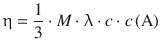
(5.17)
We can thus predict that:
✵ Since the mean free path λ is inversely proportional to the concentration, and the concentration itself features as a factor in Eq. 5.17, the viscosity η is independent of the concentration, and thus also of the pressure.
✵ The mean speed c increases with increasing temperature, and so does the viscosity η. At higher temperatures, gases have a higher viscosity.
This behaviour is in contrary to observations with a liquid: for a molecule in a liquid to move it must overcome intermolecular interactions. With increasing temperature, more molecules acquire this energy and can move; the viscosity of a liquid thus decreases with increasing temperature.