Physical Chemistry Essentials - Hofmann A. 2018

Molecules in Motion
5.2 Molecular Motion in Liquid Solutions

We have seen in Sect. 4.1.4 that ions can be dragged through a liquid solvent by applying a potential difference ΔE between two opposing electrodes. From the potential difference ΔE over a distance l, we defined the electric field as

(4.11)

The fundamental property that characterises the ability of ions to move through the solution is the resistance R (see Sect. 4.1.5); the higher the resistance, the harder it is for the ions to migrate. The conductance G of a solution is the inverse of the resistance. Therefore, the lower the resistance, the higher becomes the conductance and the easier it gets for ions to migrate through the solution:

(4.16)

The conductance G increases with the cross-sectional area A and decreases with the length l; as the constant of proportionality we introduced the conductivity κ:

(4.18)

If we measure the conductance of an electrolyte solution in suitable container and two fixed electrodes, then the cross-sectional area A and the length l are invariant parameters of the experimental system. The measured conductance will thus depend only on the number of charged species present solution. If we normalise the proportionality factor κ (the conductivity) with respect to the molar concentration of ions (c), we obtain a property that is a characteristic constant for a particular ion. This constant is called the molar conductivity Λ_m:

(5.18)

5.2.1 Conductivities of Electrolyte Solutions

In extensive measurements with strong electrolytes (substances that are fully dissociated in solution), Friedrich Kohlrausch found in the nineteenth century that at low concentrations, the molar conductivities vary with the square root of the concentration:

(5.19)

which is known as Kohlrausch’s law and introduces the limiting molar conductivity Λ_0m as a maximum molar conductivity that is attained only at indefinite dilution. The dependence on , rather than c, is due to inter-ionic interactions. While migrating, ions of a particular charge may pass ions of opposite charge and thus retard their migration. Kohlrausch’s law is only valid for strong electrolytes and describes the non-linear decrease of the molar conductivity with increasing concentration.

For weak electrolytes (which only dissociate partially in solution), the molar conductivity depends strongly on concentration. The more dilute a solution, the greater its molar conductivity, due to the increased ionic dissociation (see Fig. 5.3). The degree of dissociation α (see Sect. 4.3.3) can be obtained from the ratio of the molar and limiting molar conductivities:

(5.20)

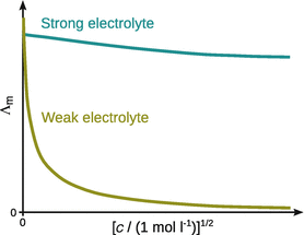
Fig. 5.3

The molar conductivities of strong and weak electrolytes increase with decreasing concentrations, but to different extents. The molar conductivity at infinite dilution is the limiting molar conductivity Λ_0m

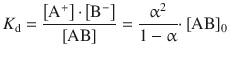
The dissociation constant K _d of weak electrolytes is related to the degree of dissociation by Ostwald’s dilution law:

(5.21)

where [A⁺], [B⁻] and [AB] are the equilibrium concentrations of the cation, anion and nondissociated electrolyte, respectively. [AB]₀ is the total concentration of electrolyte. Considering Eq. 5.20, Ostwald’s dilution law can also be expressed in the form of molar conductivities:

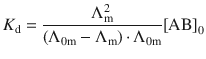
(5.22)

Experimentally, it could also be shown that the limiting molar conductivity (Λ_0m) is comprised of the two independent limiting molar conductivities of the anions (λ_-) and cations (λ₊):

(5.23)

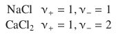
This finding is also known as the law of the independent migration of ions. In Eq. 5.23, ν denotes the number of ions per formula. For example:

5.2.2 Mobilities of Ions

In an electric field , where the two electrodes are at a distance dx = l, a particle with the charge Q = z·e experiences the force:

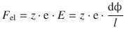
(5.24)

The particle is thus accelerated towards the appropriate electrode, but it has to overcome friction in the liquid medium. According to Stokes’ law of friction, the frictional force F _fr of a spherical particle with radius r is related to its velocity v by

(5.25)

Here, η is the viscosity of the solvent, which we have introduced in Sect. 5.1.6.

Since both forces, the electrostatic attraction and the frictional force, act in opposite direction, the final drift speed of the moving particle is established, when both forces balance each other (i.e. no net force):

(5.26)

In the above equation, we substitute the expressions from 5.24 and the left, and 5.25 on the right hand side:

Resolving for the drift speed yields:

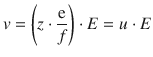
(5.27)

where u is the mobility of the ion and E the electric field the ion is exposed to.

Resolving Eq. 5.27 for u and substituting the expression for the frictional constant from above delivers an expression that links the ion mobility to the charge of the ion as well as the viscosity of the liquid medium:

(5.28)

The ion mobility u provides a link between the charge z of an ion and its conductivity λ:

(5.29)

In this equation, the constant F = N_A·e is the Faraday constant. Earlier, we have introduced the limiting molar conductivity Λ_0m as

(5.23)

where ν₊ and ν_- denote the stoichiometric number of cations and anions in the formula of the electrolyte, and λ₊ and λ_- are the conductivities of the cation and anion, respectively.

By combining Eqs. 5.23 and 5.29, we can now conclude for the limiting molar conductivity:

(5.30)

In the absence of inter-ionic interactions (i.e. at low concentrations) for a symmetrical z:z electrolyte, such as CuSO₄ (ν₊ = ν₋ = 1, z ₊ = z ₋ = z = 2) this equation simplifies to:

(5.31)

Therefore, ion mobilities are highly useful parameters in determining the limiting molar conductivities of electrolytes (Table 5.5).

Table 5.5

Limiting molar conductivity of selected ions in water at 25 °C. Note the extraordinarily high limiting conductivity of the proton and the hydroxyl ion in aqueous solution

5.2.3 Ion—Ion Interactions

In the absence of an electric field, the atmosphere surrounding a particular ion is spherical. When an ion migrates through an electric field, its atmosphere is no longer spherical but distorted, since the centres of gravity do no longer coincide. This gives rise to a reduced mobility ( relaxation). The opposite direction of the movement of ionic atmosphere and the central ion also causes a viscous drag called the electrophoretic effect (Fig. 5.4).

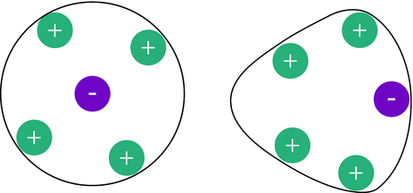
Fig. 5.4

In the absence of an electric field, the atmosphere surrounding an ion is spherical (left). However, when an ion experiences an external electric field, its surrounding atmosphere gets distorted, giving rise to reduced mobility and a viscous drag (right)

The quantitative treatment of these phenomena is complicated, but has been achieved with the Debye—Hückel—Onsager theory. This theory allows calculation of numerical values for limiting molar conductivities which are in good agreement with experimental data at low molar concentrations (mM and below). A rigorous treatment of the Debye—Hückel—Onsager theory is beyond the scope of this introduction, but we will summarise the main finding which culminates in a linear relationship between the conductivity κ and the limiting molar conductivity of an electrolyte Λ_0m:

(5.32)

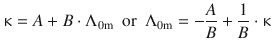
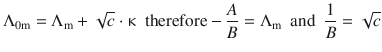
We remember that Kohlrausch’s law delivered a relationship between Λ_0m and κ that satisfies the generic expression in Eq. 5.32:

(5.19)

which can be resolved to

The theory by Debye, Hückel and Onsager yields the following expressions for the two coefficients A and B:

(5.33)

and

(5.34)

5.2.4 Diffusion

Earlier in this chapter, we have introduced diffusion as flux of matter. Since this phenomenon is of utmost importance for any chemical and biochemical process, we will extend the discussion of this particle transport and also consider some thermodynamic aspects that are linked to this transport property.

Thermodynamically, we know that if a molecule is moving from a location with the chemical potential μ₁ = μ to another location with the chemical potential μ₂ = μ + dμ, the work done by the system is dW = dμ.

In a system, where the chemical potential depends on the spatial position x, this results in a chemical potential gradient, i.e. the differential of μ with respect to . For this process, we assume constant pressure and temperature, and therefore obtain for the work dW done by the system during the diffusion:

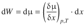
(5.35)

According to classical Newton mechanics, translocation work can generally be expressed in terms of a force opposing the direction of translocation:

(5.36)

The fact that the force F opposes the spatial translocation x results in a minus sign in the above equation. By comparison of Eqs. 5.35 and 5.36, we conclude that the force F is defined by

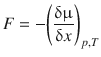
(5.37)

and is thus called the thermodynamic force. The thermodynamic force does not necessarily represent a real force that is pushing the particles down the slope of the chemical potential. It rather represents the spontaneous tendency of molecules to disperse, and thus provides a link between classical mechanics and the 2nd law of thermodynamics.

5.2.5 Fick’s First Law of Diffusion

If we now consider a solution that contains a solute of activity a, we can calculate the chemical potential of the solute as per:

(3.12)

If the solution is not uniform and the activity depends on the position x, then there exists a gradient of the chemical potential (as discussed in the previous section). From Eq. 5.37, we know that this gradient is the thermodynamic force:

(5.38)

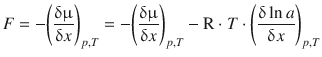
Using Eq. 3.12, the gradient can be separated into two terms, namely and . Since μ^— is the standard chemical potential it is a constant parameter and thus not dependent on the location. Its differential with respect to x is thus zero. This results in the following expression for the thermodynamic force:

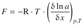
(5.39)

which we can simplify under the assumption that the solution is ideal; in that case, a = c:

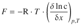
(5.40)

Using the fact that (see A.2.4), we can use the transformation of to obtain:

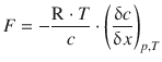
(5.41)

This equation describes the flux of diffusing particles as motion in response to a thermodynamic force which arises from the concentration gradient.

The particles reach a steady drift speed v _dr, when the thermodynamic force is matched by the viscous drag. We can then construct the following chain of conclusions:

The drift speed v _dr is proportional to the force F : v _dr ∼ F

The particle flux J is also proportional to the drift speed: J ∼ v _dr

The force F is proportional to the concentration gradient:

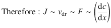
This means that the flux J is proportional to the concentration gradient; we have already come across this relationship in Sect. 5.1.4: Fick’s first law of diffusion.

From the introduction of Fick’s first law in that section, we remember that we can express the flux in terms of the concentration gradient by using the diffusion coefficient D as a constant of proportionality:

(5.10)

The flux is also related to the drift speed v _dr by:

(5.42)

Note the equality of units:

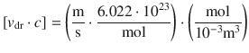
v _dr includes the Avogadro constant N_A.

By combining Eqs. 5.10 and 5.42, one obtains:

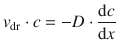
(5.43)

and from Eq. 5.41 we know that , which then yields the numerical relationship between the particle drift speed v _dr and the thermodynamic force:

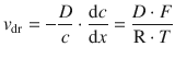
(5.44)

The constant of proportionality between the drift speed and the thermodynamic force is therefore .

5.2.6 The Einstein Relation

In Sect. 5.2.2, we discussed the mobilities of ions and derived the following expression for the ion drift speed in an electric field E:

(5.44)

In this equation, u is the mobility and the electric field.

In the case of 1 mol of ions moving through an electric field, the driving force F is the electrostatic force F _el , which is calculated according to

(5.24)

Note: ’F’ on the right hand side is the Faraday constant

Combining Eqs. 5.44 and 5.24 yields:

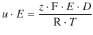
which simplifies to

(5.45)

and thus delivers an expression for the diffusion constant D as per:

(5.46)

Note: ’F’ on the right hand side is the Faraday constant

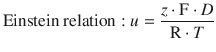
This important relationship between the diffusion coefficient D and the ion mobility u is known as the Einstein relation.

Typical ion mobilities take values at the order of u = 5·10⁻⁸ m² s⁻¹ V⁻¹for which Eq. 5.46 yields a value of D = 1·10⁻⁹ m² s⁻¹as a typical value of the diffusion coefficient of an ion in water.

5.2.7 The Stokes-Einstein Equation

We can now take advantage of the relationship between the ion mobility u and the diffusion coefficient D given by the Einstein relation and combine it with Eq. 5.28, which we derived when introducing the ion mobility in Sect. 5.2.2:

(5.45)

(5.28)

Mobility u of an ion with radius r and charge z in a medium of viscosity η

The combination of both equations yields:

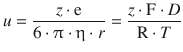
(5.47)

We then substitute the Faraday constant F = N_A·e and obtain:

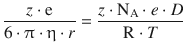
The product of charge state and elementary charge, (z·e), can be eliminated, and with the above equation becomes:

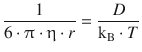
which resolves for the diffusion coefficient D as:

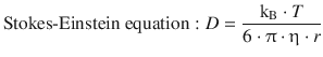
(5.48)

This equation relates the diffusion coefficient D of a solute of radius r migrating through a medium with the viscosity of that medium, η.

This important equation is called the Stokes-Einstein equation and is the basis of determination of the diffusion coefficient D by viscosity measurements. Importantly, there is no reference to the charge state of the solute, so all molecules (not just ions) can be assessed this way.