Physical Chemistry Essentials - Hofmann A. 2018
Kinetics
6.2 Reaction Rates, Rate Constants and Orders of Reaction
6.2.1 The Rate of Reaction
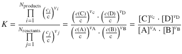
What is the rate of a reaction? Studies in the mid-nineteenth century by Cato M. Guldberg and Peter Waage led them to put forward the law of mass action (Guldberg 1864; Waage 1864; Waage and Guldberg 1864) which states that
the rate of any chemical reaction is proportional to the product of the masses of the reacting substances, with each mass raised to a power equal to the coefficient that occurs in the chemical equation:
![]()
![]()
(6.1)
After being re-discovered by van’t Hoff (1877), this law is now of historical interest, since the rate expressions derived from this law are now known to apply only to elementary reactions. However, it is still useful for obtaining the correct equilibrium equation for a reaction
(6.2)
since Guldberg and Waage recognised that chemical equilibrium is a dynamic process in which the rates of reaction for the forward and backward processes must be equal at chemical equilibrium.
In Physical Chemistry, the rate of reaction is defined as the change of concentration over time, divided by the appropriate stoichiometric coefficient. Convention describes a positive rate as a formation of products (=loss of reactants). So for the following reaction,
![]()
where A is consumed and C is produced, the reaction rate is defined as:
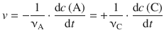
(6.3)
The rate of a reaction can be expressed with respect to different components
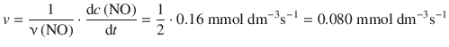
When considering the following reaction
![]()
with the formation of NO proceeding with ![]() , what is the rate of formation of NO in this reaction?
, what is the rate of formation of NO in this reaction?
For the consumption of NOBr one obtains the rate:
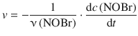
Since ![]() and ν(NOBr) = 2, this yields:
and ν(NOBr) = 2, this yields:
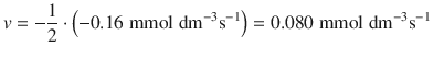
This illustrates that the rate for a reaction can be calculated with respect to any component, but always yields the same numerical value.
6.2.2 Rate Laws, Rate Constants and Reaction Order
The rate of a reaction is often proportional to the concentrations of the reactants, raised to a power:
![]()
![]()
This proportionality relationship can be transformed into an equation:
![]()
Importantly, the exponents m and n cannot be predicted a priori. In some instances, they agree with the stoichiometric coefficients (i.e. m = νA, n = νB), but in many instances this is not the case. The constant factor is called the rate constant k:
![]()
(6.4)
If m = n = 1, the units of k for this equation are:
![]()
The rate constant is independent of the concentrations of the reactants, but dependent on the temperature (see Sect. 6.5). Since the exponents m and n cannot be predicted, their values need to be determined experimentally. Equation 6.4 is thus subject to experimental verification and is called the rate law of the reaction.
The exponents m and n define the order of a reaction. A reaction with a rate law as given in Eq. 6.4 is then said to be of
✵ m-th order in A
✵ n-th order in B
✵ the overall order of (m + n)
The exponents m, n, … do not need to be integers, they can also be fractional, e.g. ![]() .
.
Some reactions obey a zero-order rate law and therefore proceed with a rate that is independent of the concentration of the reactant (as long as some is present). For example, phosphine (PH3) is catalytically decomposed on a tungsten (W) surface
![]()
and follows a zero-order reaction. In that case, the generic rate law 6.4 simplifies to:
![]()
Reactions of zero-th order are typically found when there is a limiting parameter in the reaction, such as e.g. the surface of a catalyst.
Some reactions have complicated rate laws with no overall order. For example, the formation of HBr from its elements
![]()
has the following rate equation:
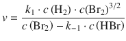
This reaction is of first order with respect to H2, but of indefinite order with respect to Br2 and HBr (see also Sect. 6.4.2).
6.2.3 Reaction Profile
Since the concentrations of reactants and products change with time during a chemical reaction, the reaction rates are often monitored experimentally by continuously measuring the concentration of a particular species during the reaction. The resulting plot that represents the change of the concentration of a species with time is called a reaction profile.
The term ’continuous’ needs to be taken with some caution. In some cases, samples are taken at various time points during a reaction and then analysed as to the concentration of a particular species (e.g. by quenching methods). Such measurements are taken at select time intervals and thus yield discrete data points. In other cases, the proceeding reaction may be monitored with a sensor (e.g. thermocouple, photodetector of a UV/Vis absorption spectrometer, etc) that delivers an electric signal which is acquired as digital data by a computer. Despite such data are often taken as continuous data, the data acquisition is not continuous but depends on the sampling rate of the analog—digital converter (i.e. consists of—a large number of—discrete data points).
The choice of the sampling rate in the experimental setting has repercussions in the mathematical treatment of kinetics (see Fig. 6.1). If a low sampling rate is applied (such as e.g. in the offline analysis/quenching method), data points are acquired spaced by long time intervals. This is called a reaction profile with discrete data points. The rates measured from various pairs of points then correspond to a mathematical Δ. Note that when graphically depicting data from discrete measurements, the appropriate choice is a scatter plot where each data point is depicted as a discrete point with a symbol (and possibly error bars, if multiple measurements are available). Discrete data points should never be connected by lines. If a mathematical model, such as a rate equation, is available, discrete data points are fitted with that equation and the fit may be superimposed as a continuous line graph on the discrete data points. The rate may then be extracted by differentiation of the underlying mathematical (fit) equation. Since the fit line is based on a mathematical equation and thus data are known for every point on the ordinate (x-axis), this constitutes truly continuous data and thus represented by connected dots (=line).
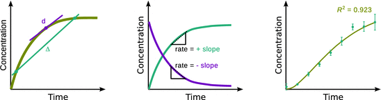
Fig. 6.1
Reaction profiles. Left: effects of low sampling rates. Centre: reaction profiles appear different, depending on whether reactant or product concentrations are followed; however, the reaction rate is the same. Right: illustration of a scatter plot and data fit
At high sampling rates, a near-continuous profile is acquired and the differences between the different data points approaches the mathematical ’d’, which is the slope of the curve at a particular point.
The left panel of Fig. 6.1 shows that a low sampling rate (turquoise) results in acquisition of discrete data points; the rates determined from discrete data points are approximations, since they represent macroscopic differences taken between two clearly distinct points (’Δ’). High sampling rates enable a near-continuous data acquisition and the rates may be determined as the slopes of tangents at any point (’d’). The centre panel of Fig. 6.1 illustrates different reaction profiles for the same reaction. Depending on whether product (turquoise) or reactant (magenta) concentrations are followed, the rate is obtained either as the positive or the negative slope from the reaction profile. The right panel of Fig. 6.1 illustrates a scatter plot of discrete data for a chemical reaction. Multiple independent measurements at individual time points allow calculation of the mean (black dots) and the estimated standard deviation (shown as positive and negative error bars). Data fitting with an appropriate rate equation results in a truly continuous reaction profile from which rates can be determined by differentiation of the underlying rate law. The goodness of fit needs to be indicated (here illustrated as an R 2 evaluation).