Physical Chemistry Essentials - Hofmann A. 2018
Kinetics
6.3 Rate Equations
A summary of the differential and integrated rate equations for the different reaction orders, along with their derived half-lives is given in Table 1.11.
6.3.1 Differential Rate Equation
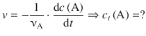
For the reaction
![]()
The rate law of the form
![]()
can be expressed as

(6.5)
which constitutes the differential form of the rate equation.
The exponent in the rate law, m, determines the order of the reaction; it is said to proceed with the m-th order. The differential rate equations for the different reaction orders are:
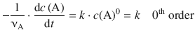
(6.6)
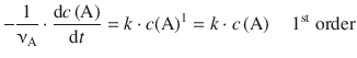
(6.7)
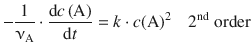
(6.8)
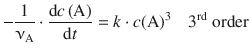
(6.9)
6.3.2 Integrated Rate Expression for the First Order Rate Law
In order to derive an expression for a given rate law that allows calculation of numerical values for the concentration of a reactant over time, the differential rate expression needs to be integrated:
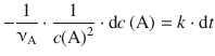
To integrate the differential 1st-order rate law
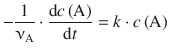
(6.7)
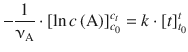
one first identifies the two variables that are of interest for the integration; here, these are c(A) and t. The equation is then re-arranged such that the two variables get isolated on opposite sides:
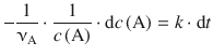
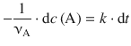
The integration has to be carried out with respect to the two differential variables, i.e. ![]() on the left side and dt on the right side. The factors
on the left side and dt on the right side. The factors ![]() and k are constants with respect to the integration and thus can be taken outside the integral. In order to calculate determined integrals, one also needs to specify the boundaries within which the integration is supposed to happen. We start at time t 0 where the concentration of A is the initial concentration c 0(A), and proceed up to time t, where the concentration of A is c t (A):
and k are constants with respect to the integration and thus can be taken outside the integral. In order to calculate determined integrals, one also needs to specify the boundaries within which the integration is supposed to happen. We start at time t 0 where the concentration of A is the initial concentration c 0(A), and proceed up to time t, where the concentration of A is c t (A):
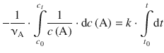
(6.10)
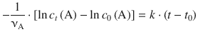
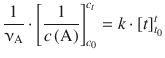
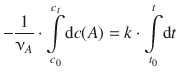
The integral on the left side, ![]() , corresponds to the type ∫x −1dx and is resolved to lnx. On the right hand side, ∫dt is of the type ∫dx which resolves to x (see Table A.2). Equation 6.10 with determined integrals thus yields:
, corresponds to the type ∫x −1dx and is resolved to lnx. On the right hand side, ∫dt is of the type ∫dx which resolves to x (see Table A.2). Equation 6.10 with determined integrals thus yields:
(6.11)
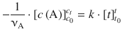
The expressions of the resolved integrals ![]() need to be calculated as per:
need to be calculated as per:
![]()
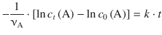
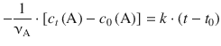
Equation 6.11 then yields:
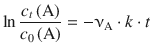
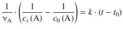
With t 0 = 0 one obtains:
In order to calculate a numerical value for the only unknown, c t (A), we isolate the expression for c t (A) on one side:
![]()
(6.12)
![]()
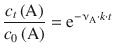
(6.13)
Equation 6.13 shows that if we measure the concentration of A, c t (A), at various time points t, and plot ln c t (A) versus t, we obtain a line with a negative slope, (−νA·k), and a y-intercept of ln c 0(A) (Fig. 6.2). Linear relationships in x—y plots are a convenient way of analysing data, and historically (before the advent of the computer) the only way to determine numerical values of fitting constants.
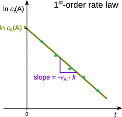
Fig. 6.2
Analysis of 1st-order kinetics by means of linear regression
With modern fitting software, it is, of course, possible to fit non-linear relationships. If Eq. 6.12 is resolved for c t (A), one obtains:
(6.14)
![]()
(6.15)
A closer look at Eqs. 6.13 and 6.15 reveals that the experimentally determined rate constant is indeed (νA·k) and includes the stoichiometric coefficient! This needs to be taken into account when calculating the rate constant k from experimental data.
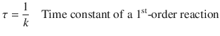
6.3.3 Half-lives and Time Constants
Half-lives and time constants are secondary parameters derived from the rate equations and can be calculated for reactions of any order.
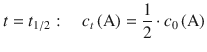
The half-life t 1/2 describes the time required to reduce the concentration of a reactant to 1/2 of its initial value. The time constant τ describes the time required to reduce the concentration of a reactant to ![]() of its initial value.
of its initial value.
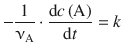
For 1st-order chemical reactions, the half-life and time constant are particularly useful indicators for the rate of the reaction, since with 1st-order reactions the two parameters do not depend on the initial concentration of reactants is the half-life t 1/2 of a reactant.
In order to derive an expression for half-life of a 1st-order reaction, we consider its definition:
![]()
Using this relationship in the 1st-order rate Eq. 4.13 yields:
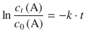
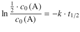
Making use of a logarithm rule that multiplies (−1) into the argument of the logarithm yields:
![]()
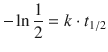
and thus
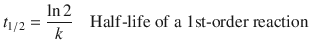
Irrespective of the initial concentration, the time it takes in a 1st-order reaction to reduce the initial concentration to half its value is always ![]() .
.
Earlier, we have introduced the time constant τ of a reaction as the time it takes for the concentration of a reactant to fall to ![]() (e ≈ 2.71828) of its initial value. As above in the case of the half-life, we use this relationship and apply it to the 1st-order rate law 4.13 which yields:
(e ≈ 2.71828) of its initial value. As above in the case of the half-life, we use this relationship and apply it to the 1st-order rate law 4.13 which yields:
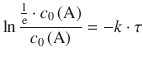

![]()
![]()
(6.17)
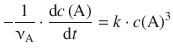
6.3.4 Integrated Rate Expression for the Second Order Rate Law
The differential 2nd-order rate law is given by Eq. 6.8:

(6.8)
We re-arrange the equation such that the two variables c(A) and t get isolated on opposite sides:
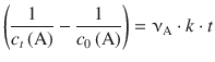
and integrate from time t0 where the concentration of A is c 0 (A) to time t, where the concentration of A is c t (A):

(6.18)
The integral on the left side, ![]() corresponds to the type ∫x −2dx and is resolved to
corresponds to the type ∫x −2dx and is resolved to ![]() . On the right hand side, ∫dt is of the type ∫dx which resolves to x (see Table A.2). Equation 6.18 with determined integrals thus yields:
. On the right hand side, ∫dt is of the type ∫dx which resolves to x (see Table A.2). Equation 6.18 with determined integrals thus yields:
With t 0 = 0, this yields:
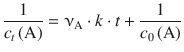
(6.19)
or, when resolving for c t (A):
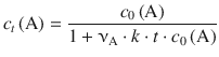
(6.20)
Equation 6.19 shows that for the second order rate law, a linear correlation is obtained when plotting ![]() versus t, where the slope is νA ⋅ k and the y-intercept is
versus t, where the slope is νA ⋅ k and the y-intercept is ![]() (Fig. 6.3).
(Fig. 6.3).
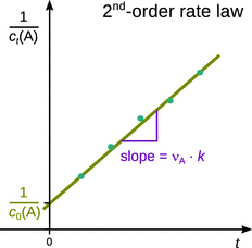
Fig. 6.3
Analysis of 2nd-order kinetics by means of linear regression
6.3.5 Integrated Rate Expression for the Third Order Rate Law
The differential 3rd-order rate law is given by Eq. 6.9:
(6.9)
For integration, we again isolate the two variables, c(A) and t, on opposite sides:
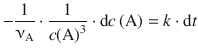
and integrate from [t 0 , c 0 (A)] to [t, c t (A)]:
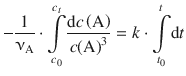
(6.21)
The integral on the left side, ![]() corresponds to the type ∫x −3dx and is resolved to
corresponds to the type ∫x −3dx and is resolved to ![]() . On the right hand side,
. On the right hand side, ![]() is of the type ∫dx which resolves to x (see Table A.2). Equation 6.21 with determined integrals thus yields:
is of the type ∫dx which resolves to x (see Table A.2). Equation 6.21 with determined integrals thus yields:
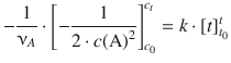
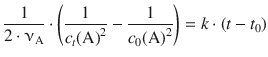
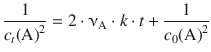
(6.22)
Therefore, a plot of ![]() against t will yield a line with slope 2 ⋅ νA ⋅ k and intercept
against t will yield a line with slope 2 ⋅ νA ⋅ k and intercept ![]() (Fig. 6.4).
(Fig. 6.4).
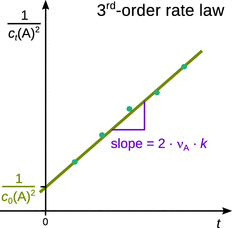
Fig. 6.4
Analysis of 3rd-order kinetics by means of linear regression
6.3.6 Integrated Rate Expression for the Zero-th Order Rate Law
In order to integrate the differential rate law of zero-th order
(6.6)
the two variables, c(A) and t, are isolated on opposite sides of the equation:
We then integrate from [t 0 ,c 0 (A)] to [t, c t (A)]:
(6.23)
The integrals on both sides side,  and
and ![]() , correspond to the type ∫dx which resolves to x (see Table A.2). Equation 6.23 with determined integrals thus yields:
, correspond to the type ∫dx which resolves to x (see Table A.2). Equation 6.23 with determined integrals thus yields:
which results in
With t 0 = 0 this yields:
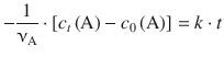
![]()
![]()
(6.24)
Therefore, a plot of c t (A) against t will yield a line with slope −νA ⋅ k and intercept c 0(A) (Fig. 6.5).
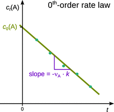
Fig. 6.5
Analysis of 0th-order kinetics by means of linear regression