Physical Chemistry Essentials - Hofmann A. 2018

Kinetics
6.4 Determination of the Rate Law

6.4.1 Analysing Data Using the Integrated Rate Laws

If kinetic data for a chemical reaction have been obtained, there are two ways to check whether the reaction adheres to any of the standard rate laws (0th—3rd order).

If at least two data points, t and c _t (A), are known, one can substitute these values into the four integrated rate laws (Eqs. 6.24, 6.15, 6.19 and 6.22) and estimate the rate constants k for the different orders. For the correct order, the two data points need to yield the same value for the rate constant.

Alternatively, the linear relationships (Eqs. 6.24, 6.13, 6.19 and 6.22) of the integrated rate equations can be plotted and subjected to a linear fit (see Figs. 6.2, 6.3, 6.4, and 6.5). The rate law that produces the best fit is likely to be the right one (Table 6.1).

Table 6.1

The rate law may be determined by graphical representation of data and checking for a linear relationship. The rate constant is then obtained from the slope

Importantly, the experimentally determined rate constant k _exp as obtained from the slope of these linear relationships is related to the ’true’ rate constant k by a proportionality factor that also depends on the stoichiometric coefficients of the reaction.

6.4.2 Experimental Design: Isolation Method

Given the reaction

with the general rate law

(6.4)

we are now concerned with experimental approaches that allow determination of the exponents m, n, etc.

In the isolation method, all starting reactants are supplied in excess except for one (e.g. reactant A). One can then assume that all excessively supplied reactants remain approximately at their initial concentration; the one component with limited supply is ’isolated’. In the above example, one can then assume for B that:

For the rate law (Eq. 6.4), it follows that

The rate constant k and the constant factor c ₀ (B) ⁿ can be combined to an apparent rate constant k′:

(6.25)

This resulting rate law only features the concentration of one component (the isolated reactant) and is thus called a pseudo-1st-order rate law.

In order to exploit the pseudo-1st-order rate law in such a way, one needs to determine the rate of a reaction at a given time t, as well as the concentration of A at that particular time t. The most frequently used approach in this context is to just consider the initial rates, i.e. the rate at time t = 0. This eliminates the need to re-examine the concentration of A, as it will be essentially the starting concentration of the reactant, c ₀(A). In the method of initial rates, the rate is thus measured at the very beginning of the reaction when the concentration of the reactants is still at their initial values. Equation 6.25 then becomes:

and by subjecting the equation to a logarithmic transformation (and using the logarithm rule of log(a ⋅ b) = log a + log b), one obtains:

With the rule of log a ^m = m ⋅ log a this yields:

(6.26)

Experimentally, the initial rates are determined for a series of different initial concentrations of A. A plot of logv ₀ versus logc ₀(A) then results in a line with slope m and intercept log k′_A (see Fig. 6.6).

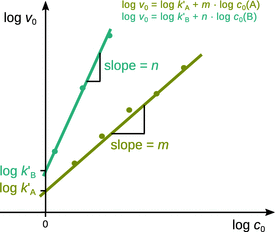
Fig. 6.6

Determination of the reaction order using the isolation method on initial rates

Using this pseudo-1st-order rate law, the exponent of the isolated reactant can be obtained and thus the true order of the reaction with respect to this reactant may be established. Subsequently, all other starting reactants are isolated, one at a time, thus allowing conclusions as to the remaining reaction orders.

A caveat for the method of initial rates

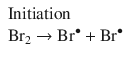
The method of initial rates may not always reveal the full rate law. Reaction products may participate in the reaction and thus affect the rate. As first proposed in 1907 (Bodenstein and Lind 1907), in the reaction that synthesises HBr from H₂ and Br₂

the product HBr engages in the radical reaction mechanism (which consists of consecutive elementary reactions; see Sect. 6.6):

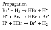
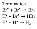
Based on this reaction mechanism, the following rate equation is derived:

6.4.3 Reactions Approaching Equilibrium

In practice, kinetic studies often conducted immediately after initiation of a reaction, i.e. far from the equilibrium. Therefore, reverse reactions need not be considered and the method of initial rates may be applied. However, when a reaction actually approaches equilibrium, the concentrations of products have to be taken into account. As an exemplary case, we consider a chemical equilibrium

(6.27)

where both the forward and reverse reactions follow a 1st-order rate law (which is, for example, the case in some isomerisation reactions).

The concentration of A is thus decreased by the forward reaction, but increased by the reverse reaction, and one obtains the following rate expression:

(6.28)

With

we can substitute c(B) in Eq. 6.28 and obtain:

(6.29)

The integrated form of the differential Eq. 6.29 resolves to:

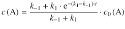
(6.30)

From Eq. 6.30, one can calculate the equilibrium concentration of A by considering a very large value for the time t; if the reaction is allowed to continue for a long time, it will certainly have reached equilibrium. With knowledge of the function e^−x (see Fig. 6.7) it becomes clear that:

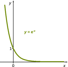
Fig. 6.7

The function e^−x anneals to zero when x takes very large values

Therefore, the term in Eq. 6.30 can be neglected and the equilibrium concentration of A resolves to:

(6.31)

For the equilibrium concentration of B, one obtains:

(6.32)

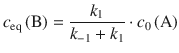
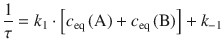
As illustrated in Fig. 6.8, in the course of the reaction, the concentration of A decreases over time and attains its equilibrium value once the equilibrium has been reached. In turn, the concentration of B increases over time up to the value of its equilibrium concentration. Importantly, at equilibrium the rates of the forward and reverse reactions are the same. We can thus conclude:

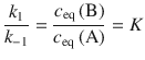
(6.33)

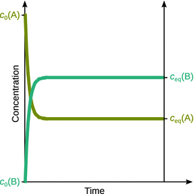
Fig. 6.8

Time-dependent development of the concentrations of A and B in reaction 6.27

This relationship provides a link between the equilibrium constant of the reaction, K (see Eq. 6.2), a thermodynamic quantity, and the rate constants, k ₁ and k ₋₁, which are kinetic properties.

6.4.4 Relaxation Methods

When a system is disturbed and thus taken off equilibrium conditions, the term relaxation refers to the return to a state of equilibrium. When a chemical reaction is at equilibrium, and environmental parameters such as temperature or pressure are suddenly changed, the system will adjust itself to new equilibrium conditions (cf. Le Châtelier’s principle; Sect. 6.1.2).

Manfred Eigen (1967 Nobel Prize in Chemistry) developed methodologies in the 1950s to experimentally determine rate constants of fast reactions based on these phenomena (Eigen et al. 1953; Eigen 1954). Technically, it is possible to elicit sudden changes in temperature ( T-jump) or pressure ( p-jump). If a reaction has a definite reaction enthalpy Δ_rH (Δ_rH ≠ 0), the equilibrium constant K of that reaction is dependent on the temperature (van’t Hoff equation, Eqs. 2.60, 2.61 in Sect. 2.2.6). In response to a sudden temperature change (T-jump), the reaction will respond by a relaxation process that established the new equilibrium based on the new temperature. Similarly, if the reaction volume Δ_rV has a definite value (Δ_rV ≠ 0), then its equilibrium constant is dependent on the pressure. A sudden pressure change (p-jump) will result in a relaxation that adjusts the equilibrium to the new conditions.

Irrespective of the order of the underlying reaction, the relaxation process will follow a 1st-order kinetics.

Since the equilibrium composition of a reaction depends on the temperature or pressure, the concentrations of the individual components after a T- or p-jump will differ from the equilibrium concentrations c _eq(A), c _eq(B) and c _eq(C) by a concentration difference Δ_jumpc. For the simple equilibrium

this means

Without rigorously deriving the consequences here, it can be shown that the change of the concentration difference Δ_jumpc with time occurs as per

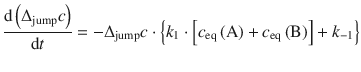
After separation of variables and integration, this leads to the relationship

(6.34)

In Eq. 6.34, Δ_jumpc(t) is the concentration change at time t, and Δ_jumpc(0) the concentration change immediately after the T/p-jump. By comparison, we find that this equation takes the form of equation

(6.15)

which describes a 1st-order kinetics.

The time constant τ of a first order reaction as then as per Eq. 6.17:

Note: k is the true rate constant from Eq. 6.15.

Applied to Eq. 6.34 for the relaxation after a T/p-jump, the time constant becomes:

By using the relationship , this can be transformed to:

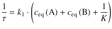
(6.35)

Due to the system relaxing after a T/p-jump, the time constant τ is now called relaxation time.

T-jump and p-jump experiments therefore offer a way to determine rate constants of the forward and reverse reactions of an equilibrium. If the equilibrium constant is known, a single measurement of the relaxation time τ can reveal the values for k ₁ and k ₋₁.

6.4.5 Monitoring the Progress of a Reaction

The rates of chemical reactions are measured using techniques that monitor the concentrations of species present in the reaction mixture. Moderately fast reactions can be monitored by ’freezing’ the state of a reaction at a certain time—a method called quenching. The quenched reaction can then be analysed offline, using a suitable experimental procedure. Fast reactions often require real-time analysis or the application of relaxation methods (see previous section). We will look at some experimental methodologies for both cases in Sects. 6.4.6 and 6.4.7.

Importantly, the time scale of a particular reaction often does not solely depend on the value of the rate constant. Only for 1st-order reactions does the half-life t _1/2 depend exclusively on the rate constant k:

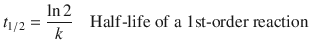
(6.16)

For 2nd- and 3rd-order reactions, the half-lives depend on the concentration of the reactants as per:

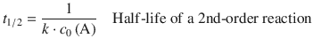
(6.36)

(6.37)

and such reactions can thus be slowed down by choosing lesser initial concentrations. However, the accuracy of concentration measurements decreases as concentrations become smaller, and therefore there will be technical limits. For reactions that follow 0th-order, the half-life is

(6.38)

So in order to increase the half-life in such cases, larger initial concentrations are required.

A reaction where at least one component is a gas might result in an overall change of pressure in a system of constant volume. Such reactions may be followed by recording the variation of pressure with time. Spectrophotometry is a widely applicable technique; it measures the absorption of electromagnetic radiation and is particularly useful, if a component in the reaction mixture has characteristic spectral properties. Reactions where the number or type of ions change can be monitored by recording the electric conductivity. If hydrogen ions are produced or consumed during a reaction, its progress can be followed by monitoring the pH of the solution.

Examples of monitoring reaction kinetics

1. (1)

This gas phase reaction may be monitored by absorption of visual light by Br₂. The visual absorption maximum of Br₂ is at λ_max = 420 nm (Hubinger and Nee 1995).

1. (2)

Here, the conductivity or pH of the solution may be monitored.

1. (3)

The kinetics of the alkaline hydrolysis of acetylsalicylic acid (aspirin) in solution can be analysed by quenching the reaction mixture at various time points and determining the amount of hydroxyl ions remaining at that time by back-titration.

Alternatively, the reaction may be monitored by UV/Vis spectroscopy. The product of the reaction, salicylic acid/salicylate, possesses an absorption maximum at λ_max = 298 nm; acetylsalicylic acid has no significant absorbance at this wavelength.

1. (4)

The reaction of hydrogen peroxide with iodide in acid solution is a fast exothermic reaction. The kinetics of this process can be monitored via the released heat output, i.e. in terms of temperature rise. This can be done with a calorimeter.

6.4.6 Experimental Techniques for Moderately Fast Reactions

In order to achieve homogeneous mixing of reactants at the beginning of a reaction, the experimental challenges increase with increase of the reaction rate. With moderately fast reactions (half-lives at the order of seconds), conventional mixing techniques are quite appropriate. Typically, such reactions are started by addition of one of the reactants to a stirred solution containing the remaining reactants.

Data acquisition may either occur using a real-time technique (e.g. pH electrode, recording of absorbance) or by stopping the reaction at various time points (quenching) and analysing the concentration of reactants with a suitable protocol. There are three types of quenching methods:

Conventional Quenching

Here, the reaction is stopped after it has been allowed to progress for a certain time. Reaction intermediates may be trapped and analysis can proceed at any time. This works for reactions that are slow enough such that there is negligible reaction going on during the quenching process.

Freeze Quench Method

Here, the reaction is quenched by rapid cooling of the mixture. Concentrations of reactants, intermediates and products can then be measured.

Chemical Quench Flow Method

Reactants are mixed as in the flow method (see next section). The reaction is quenched by another reagent (e.g. acid, base) after the mixture travelled along a fixed length through the outlet tube. Once the reaction has been quenched, analysis of concentrations can proceed with any suitable “slow” method.

6.4.7 Experimental Techniques for Fast Reactions

For fast reactions, mixing of reactants at the start of the reaction needs to be achieved by flow methods. Here, reactants are mixed rapidly as they are introduced into a chamber. The reaction continues while the mixture flows through the outlet tube. Two types of flow methods are commonly in use: the continuous flow and the stopped flow (see Fig. 6.9).

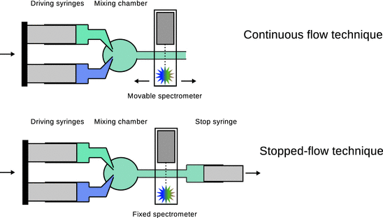
Fig. 6.9

Schematic comparison of the experimental setup for continuous flow (top) and stopped flow (bottom)

With exception of the chemical quench flow method (see previous section), data acquisition in flow methods is typically by real time methods, whereby either a small sample is withdrawn or the bulk reaction mixture is monitored. Figure 6.10 shows a stopped flow instrument with an integrated absorbance spectrometer.

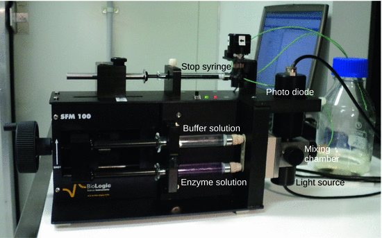
Fig. 6.10

A stopped flow UV/Vis absorption spectrometer

Enzymatic activity of carbonic anhydrase by stopped-flow kinetics

Carbonic anhydrases are essential enzymes in all organisms regulating CO₂ but also pH homeostasis. They catalyse the (de-)hydration of CO₂:

In the forward direction, the environmental pH is lowered, in the reverse direction, the pH is increased. This pH change, which is due to the production of 1 mol H⁺ for each mol CO₂ consumed, allows monitoring of the reaction (Khalifah 1971). For stopped-flow experimentation, this is done by a pH indicator whose colour change is monitored spectrophotometrically (compared to the fast reaction, pH electrodes require too long to equilibrate for a stable read-out). The pH indicator used at mildly acidic pH is m-cresol purple; its spectral characteristics at different pH conditions are shown in Fig. 6.11. m-cresol purple has an absorption band at λ_max = 578 nm; the absorbance decreases with decreasing pH. The indicator in the reaction mix thus allows monitoring of H⁺ production and, therefore, CO₂ consumption.

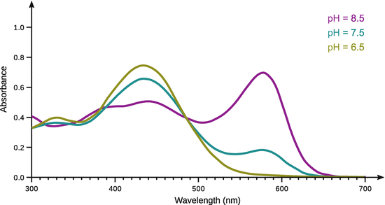
Fig. 6.11

Absorption spectra of m-cresol purple in the visual range at different pH conditions (6.5, 7.5, 8.5)

Figure 6.12 shows a reaction profile obtained by stopped-flow kinetics experiments with human carbonic anhydrase II. Note that the reaction has finished after 80 ms!

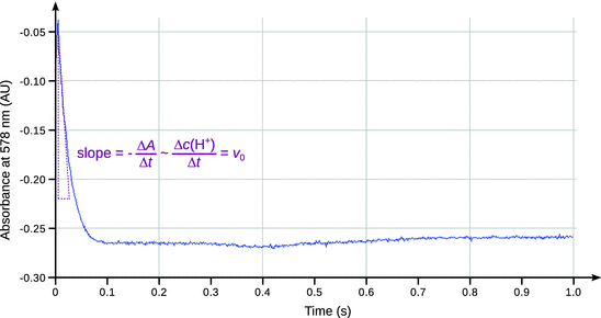
Fig. 6.12

Reaction profile of human carbonic anhydrase II from a stopped flow kinetics assay using m-cresol purple as indicator