Physical Chemistry Essentials - Hofmann A. 2018

The Fabric of Atoms
8.3 Introduction to Quantum Mechanics

8.3.1 The Schrödinger Equation

Whereas the planet-like model chosen by Bohr can easily be visualised and is thus a fairly accessible model, the postulates required to achieve agreement with experimental observations are not immediately accessible. The general problem with this approach is the direct application of macroscopic laws to processes at the atomic level.

A different concept was suggested by Erwin Schrödinger based on the dualism of wave and matter, giving rise to the so-called wave mechanics. In that context, we have previously introduced the wave function Ψ which describes matter as a wave and as such does not require an individual point in space and time for characterisation. It has also become clear that the squared amplitude, Ψ², is a measure of the probability to find a particle in a volume element of space. In order to learn about states in atoms, it will be sufficient to analyse the wave function Ψ for its properties in various locations, i.e. Ψ(x, y, z). If we are dealing with processes such as radiation, however, the time time-dependence of the wave function will also need to be considered, i.e. Ψ(x, y, z, t).

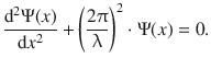
For instances independent of time, Schrödinger suggested the following equation for the wave function Ψ(x, y, z) in three dimensions

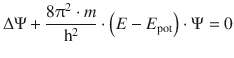
(8.24)

Notably, this equation cannot be proven from first principles. Very much like the laws of thermodynamics, the equation is a description of naturally occurring phenomena, whose ’proof’ is the fact that it correctly describes these phenomena.

In Eq. 8.24, ’Δ’ does not indicate a difference, but rather the Laplace operator which describes the second derivative:

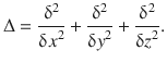
(8.25)

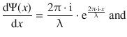
For simplicity, we will reduce further discussion of this problem to just one dimension (x). Visually, this suggests that we are dealing with a standing wave (Fig. 8.10). The mathematical expression for such a wave (cf. harmonic oscillator) is:

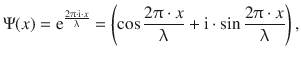
(8.26)

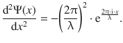
where x is the coordinate in space (one dimension), λ is the wavelength and i is defined as per i² = −1. Calculation of the first and second derivative of the expression for the one-dimensional wave Ψ(x) yields:

(8.27)

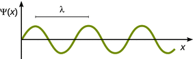
Fig. 8.10

Illustration of a one-dimensional standing wave

The expression for the second derivative can be re-arranged to read:

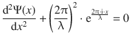
(8.28)

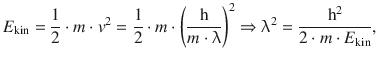
From the DeBroglie relationship (Eq. 8.10), we can derive that

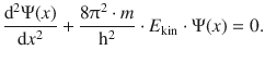
and then can obtain an expression for the kinetic energy E _kin that can be resolved for λ²:

and the above expression can be substituted in the wave Eq. 8.28:

Since the total energy of a particle is the sum of its kinetic and potential energy (E = E _kin + E _pot), we obtain:

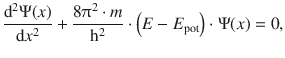
(8.29)

and find that Eq. 8.29 is the one-dimensional form of the Schrödinger Eq. 8.24. Importantly, this agreement itself is not proof that the Schrödinger equation is correct.

Conceptually, the use of this equation for quantum mechanical problems assumes a model whereby particles with a mass m can be described as waves of matter. This raises the question of what exactly is propagating through space in a wave of matter. This question was answered by Max Born in 1928 who interpreted waves of matter as probability waves. Intriguingly, quantum mechanics therefore is intrinsically probabilistic. Whereas in classical mechanics, one can assign precise coordinates to a particle (limited only by the instrumentation used for measurement), quantum mechanics only allows assignment of probabilities to find a particle in one volume element or another. The Schrödinger equation acts as the link between both of these ’worlds’. The particles possess a potential energy E _pot and a mass m both of which can be determined using physical laws of the macroscopic world. Based on these numerical values the Schrödinger equation delivers the wave function Ψ and the total energy E which describe the quantum mechanical behaviour of the particle.

8.3.2 Basic Properties of Wave Functions

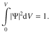
We will find later that wave functions can be determined with exception of a constant factor (Sect. 9.1.1, Eq. 9.3). However, since we concluded that the squared amplitude of the wave function is a measure of the probability to find the particle in a volume element dV, then the total probability to find the particle somewhere has to equal one. Mathematically, the total probability corresponds to an integration of the function |Ψ|² over the entire volume V:

(8.30)

The constant factor will thus have to be set such, that Eq. 8.30 is adhered to. In that case, the wave function Ψ is called a normalised wave function. A close look at the above equation shows that |Ψ|² carries the units of probability per volume and therefore constitutes a probability density.

The reason we have now introduced |Ψ|² instead of Ψ² for the probability density is that wave functions will involve complex numbers (as opposed to real numbers), in which the case the square amplitude is computed as the product of the amplitude and its complex conjugated:

(8.31)

Complex numbers consist of a real (ℜ) and an imaginary (ℑ) part: C = ℜ + i ⋅ ℑ The complex conjugate of C is defined as C ^∗ = ℜ − i ⋅ ℑ. It is thus obvious that the product of C and C* yields the sum of the squared real and imaginary parts:

If the imaginary part is zero (ℑ = 0) then C is a real number and the square operation reduces to the case well-known for real numbers:

Above, we came to appreciate that in order for |Ψ|² to assume a physical meaning, we require the wave function Ψ to adhere to Eq. 8.30. Therefore, the function Ψ has to fulfil the following pre-requisites:

✵ Ψ needs to be a continuous function and we need to be able to determine its derivative. This requires that the first and second derivative of Ψ are also continuous functions. In other words, Ψ must not have any kinks are jumps.

✵ Ψ has to be unambiguous; for a particular set of values of the independent variables (x, y, z, t), there has to be only one value of Ψ.

✵ Ψ needs to assume finite values throughout and approach values of zero when the spatial variables x, y and z become infinite.

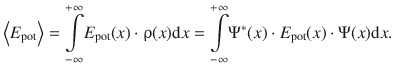
It is frequently necessary to calculate properties of a particle or system that are not immediately obtained by solving the Schrödinger equation. Obvious examples are the potential energy E _pot or the momentum p of a particle that are not directly available from the Schrödinger equation which only allows direct calculation of the total energy E.

In order to outline the general procedure for such cases, we will, for simplicity, again consider a one-dimensional wave function Ψ(x). The probability density function ρ(x) is given based on Eq. 8.31:

(8.32)

The probability to find the particle in the interval x and x + dx is then available via the integral . Therefore, if we are interested in the average value of the potential energy E _pot , which itself is a function of the location x, the function E _pot(x) needs to be multiplied with the probability ρ(x) to find the particle at each location x, and then integrate over all location values x. In this context (of probability theory), the average value of a quantity (e.g. ) is called the expected value of this quantity, denoted as <E _pot>: