Physical Chemistry Essentials - Hofmann A. 2018

Quantum Mechanics of Simple Systems
9.1 The Particle in a Box

9.1.1 The Free Particle

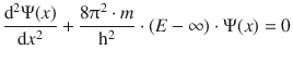
As a first application of the Schrödinger equation, we will characterise a free particle that exists in space without any potential (E _pot = 0). For convenience, we will also consider just one dimension. Given these conditions, the Schrödinger equation 8.28 becomes

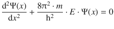
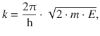
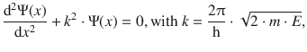
For simplicity, we introduced the parameter k to substitute the factor containing the mass of the particle (m), its energy (E) and the constants:

(9.1)

which yields

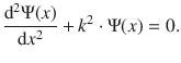
(9.2)

If we assume that the wave function is Ψ(x) = e^{b ⋅ x}, then the second derivative of Ψ(x) is d²Ψ(x) = b ² ⋅ e^{b ⋅ x}. Substitution of those values in Eq. 9.2 yields:

Since the function e ^b·x never assumes the value of zero, the above equation is only true if:

For this quadratic equation, two solutions are possible. We also remember that b might be a complex number, and therefore obtain:

This results in two solutions for the wave function:

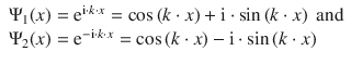
Using these two partial solutions, we one can solve the differential Eq. 9.2. Without performing this mathematical exercise in a rigorous fashion, we appreciate that the general solution for a wave function fulfilling Eq. 9.2 is:

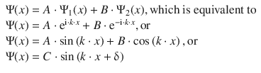
(9.3)

where A, B, C and δ are constants resulting from the integration required when solving the differential Eq. 9.2.

It can be shown that for B = 0, the particle possesses a momentum that is positive with respect to the x-axis, i.e. it moves along the direction of the positive x-axis branch. In contrast, for A = 0, the momentum is negative, indicating that the particle moves in the direction of the negative x-axis branch. Inspection of the general solution of the wave function, e.g. in the form of

(9.3)

shows that Ψ is the superposition of two sine-like waves. The two waves are running in opposite directions and, by interference, result in a standing wave.

In the above discussion, it has not been necessary to demand any particular values for the parameter k. Upon re-arrangement of Eq. 9.1, we obtain the energy E of the particle:

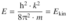
which constitutes the kinetic energy of this particle, since we set out with the requirement that the potential energy was zero. Since k can assume any value, the kinetic energy of the free particle can assume any value—it exists in a continuum.

9.1.2 The Particle in a One-dimensional Box with Infinite Potential Walls

In the previous section, we introduced the general solution of the Schrödinger equation and derived a wave function that describes a freely moving particle of the kinetic energy E _kin and no potential energy (E _pot = 0).

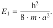
We now want to consider the case that the particle is enclosed in a box of width a in which it can move around freely (no potential energy), but from which it cannot escape. This can be realised by imposing a steeply rising potential at the walls of the box (Fig. 9.1). The potential at the walls of the boxes will be set infinitely high. Therefore, three regions need to be considered:

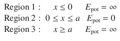
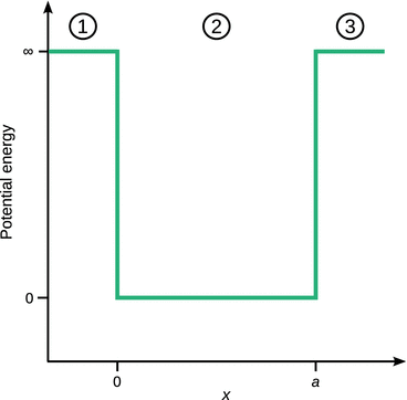
Fig. 9.1

The potential well for the particle in a box

For regions 1 and 3, the Schrödinger equation is:

This equation can only be adhered to, if the wave function is Ψ(x) = 0. Notably, this results in a probability density of ρ(x) = 0, which means that the particle does not exist in those regions:

In region II, the particle can move without restriction, since E _pot = 0. This is the same case we have discussed in the previous section. The Schrödinger equation is thus:

(9.2)

and we obtain the general solution

(9.3)

It is important to remember now that a general prerequisite for any wave function Ψ is that it is a continuous function (Sect. 8.3.2). Due to the high potential at the walls of the box, which made us conclude for Ψ(x) = 0 in regions I and III, this means that:

The condition of Ψ(x) = 0 can only be met, if in Eq. 9.3 the cosine term disappears, i.e. B = 0. The second condition, Ψ(a) = 0, requires then that

Since a sine function periodically assumes values of zero when the argument is an integer multiple of π (Fig. 9.2), the product k·a needs to fulfil the requirement:

which means that k can only take particular values:

(9.4)

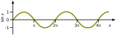
Fig. 9.2

The function sin x periodically assumes a value of zero

The allowed solutions for the Schrödinger Eq. 9.2 thus are:

Note that at this stage, only solutions with n ≠ 0 remain possible, since a wave function of Ψ₀(x) = 0 would not be a sensible solution; the particle has to be in the box. The value of A is chosen such that the wave function is normalised, and this process yields:

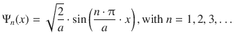
(9.5)

Importantly, the energy values that the particle in the box can assume are no longer continuous, but subject to the condition 9.4:

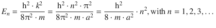
(9.6)

So whereas the freely moving particle can assume any energy value, the particle confined in a potential well (box) is only allowed to assume discrete energy values (Eq. 9.6) which are a function of the principal quantum number n. The allowed discrete energy values are called eigenvalue of the Schrödinger equation

Figure 9.3 summarises the allowed energy levels, the wave functions and probability densities for the first four quantum numbers n. It becomes obvious that the probability of finding the particle in various areas within the box is not the same at all locations x, and it also is a function of the quantum number n. The graphs of the wave functions in Fig. 9.3 illustrate that the number of knots (where the wave function assumes a value of zero) equals (n−1); note that the knots at the walls are not considered.

Fig. 9.3

Allowed energy levels E _n , wave functions Ψ _n and probability densities |Ψ _n |² for the particle in a linear potential well

Lastly, Eq. 9.6 shows, that any particle in a potential well has a minimum energy and cannot assume a state of zero energy. Since the lowest value for the quantum number is n = 1, the minimum energy is:

9.1.3 The Particle in a One-dimensional Box with Finite Potential Walls

In the previous section, the potential well was constructed with infinitely high potential such that it was impossible for the particle to leave, regardless of how much energy would be provided to the system. here, we will consider the more realistic case of potential walls with finite heights. Within the well, the particle of mass m shall not be exposed to any potential (E _pot = 0), outside the well, the particle shall be exposed to the potential energy V ₀. As before, we need to distinguish three regions:

but also two different cases with respect to the total energy E of the particle:

E < V ₀: in this case, the energy of the particle is not sufficient to leave the well. This is the case of the bound particle.

E > V ₀: here, the energy of the particle is sufficient to leave the well. However, when outside the well, it experiences the potential V ₀, in contrast to the free particle (Sect. 9.1.1).

When solving the Schrödinger equation for the different cases, it is found in agreement with the previous simpler models, that the allowed energy of the particle inside the well are discrete (Fig. 9.4 left). In addition, one observes that the number of possible energy states increases with the potential energy value V ₀ outside the well, and also with the width of the box a. And lastly, the values of the allowed energy levels (eigenvalue) increase with increasing potential V ₀.

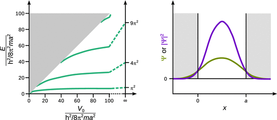
Fig. 9.4

Energy levels of a particle in a well with potential V ₀. If the total energy of the particle E is less than V ₀ (lower right half of the diagram), the particle is bound and can only assume discrete energy levels (eigenvalue). The number of the different possible levels as well as their numerical value depends on the value of V ₀ and the width of the well a. If the total energy of the particle E is larger than V ₀ (upper left half of the diagram), the particle is in an energy continuum (it may assume any energy) and no longer bound

A further notable observation of the box with finite potential walls is made when the wave functions Ψ and the probability densities |Ψ|² are analysed (Fig. 9.4 right). The solution of the Schrödinger equation in this case shows that both functions assume non-zero values outside the potential well, in contrast to the box with infinite walls (Fig. 9.3). The fact that the bound particle may also be found outside the box shows that it can exist in regions where the total energy E is less than the potential energy V ₀; this is only possible if it possesses negative kinetic energy!