Physical Chemistry Essentials - Hofmann A. 2018

Quantum Mechanics of Simple Systems
9.2 The Rigid Rotor

9.2.1 The Rigid Rotor with Space-fixed Axis

Following the introductory applications of the Schrödinger equation to individual particles, we now consider the circular movement of two masses m ₁ and m ₂ that are connected by a rigid connection—a very simple model for a two-atomic molecule. For rotational movement of a mass m, we need to consider the momentum of inertia I which is given by

(9.7)

where r is the distance of the mass to the axis of rotation. For convenience, the velocity of the mass m is given as an angular velocity ω which is related to the rotational frequency ν_rot:

(9.8)

If two connected masses m ₁ and m ₂ rotate around their centre of gravity (at distance r ₁ from mass m ₁ and at distance r ₂ from mass m ₂), the system can be substituted by one where a reduced mass μ (sometimes also called effective mass) rotates around a centre at distance r (Fig. 9.5):

(9.9)

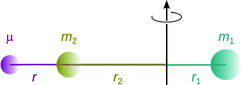
Fig. 9.5

The reduced mass μ allows substitution of a two-body rigid rotor with a one-body rigid rotor

The position of the centre of gravity is given by:

(9.10)

Combining Eqs. 9.9 and 9.10 yields the following expressions for the distances r ₁ and r ₂:

(9.11)

The momentum of inertia for the system consisting of two connected masses is then:

With Eq. 9.11 this yields:

(9.12)

and thus defines the reduced mass μ.

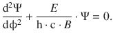
In the simplest case, a rigid rotor (r = const.) possesses a rotation axis which itself is fixed in space. The circular movement of a point around the rotation axis at distance r is then best described by monitoring the angle ϕ (measured against the positive branch of the x-axis in a Cartesian coordinate system). The location parameter describing the movement is thus chosen as (r·ϕ). If we assume that the rotor is not subject to any outside potential (E _pot = 0), the Schrödinger equation 8.28 becomes:

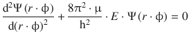
where the radius r can be isolated from the differential since the only variable in the location parameter in a given rotor is the angle ϕ:

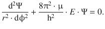
(9.13)

For further convenience it seems useful to introduce a rotational constant B which is defined as

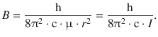
(9.14)

Eq. 9.13 then becomes

(9.15)

If we define a further constant k as

Eq. 9.15 takes the form of

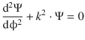
(9.16)

which we can solve immediately, recalling the general solution of the Schrödinger equation for a free particle that is not subjected to an external potential:

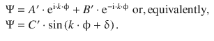
(9.17)

Sensible solutions for Eq. 9.17 are obtained when the wave function Ψ assumes the same value after a full rotation, therefore

This requirement, however, is only met, if the constant k in the Schrödinger Eq. 9.16 assumes only integer values:

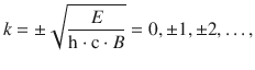
which means that the energy of the rigid rotor cannot assume any, but only discrete values (Fig. 9.6):

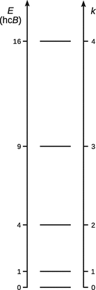
Fig. 9.6

Allowed energy levels for a rigid rotor with fixed rotation axis

9.2.2 The Rigid Rotor with Space-free Axis

The rigid rotor with space-fixed axis only rotates in a plane perpendicular the rotation axis. If we think about this as a model for an electron rotating around an atomic nucleus, in the general—and more realistic—case, the rotation plane can form any angle with the rotation axis. In addition to the two parameters r (distance of the mass from the rotation axis) and ϕ (rotational angle of the mass with respect to the positive x-axis), a third parameter needs to be considered that describes the angle of the rotational plane with the positive z-axis; this angle is called θ.

Since these three parameters uniquely describe the position of a point in the three dimensional space they can be used instead of the Cartesian coordinates x, y and z. This new coordinate system is called the spherical coordinate system consisting of

✵ r radial coordinate

✵ ϕ azimuth angle

✵ θ polar (or inclination) angle.

The transformation of spherical to Cartesian coordinates is possible by:

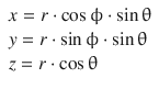
(9.18)

and graphically illustrated in Fig. 9.7.

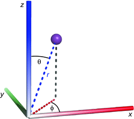
Fig. 9.7

Polar coordinates and the Cartesian coordinate system

When solving the Schrödinger equation, we now need to explicitly consider the wave function Ψ being a function of three coordinates, Ψ(r, ϕ, θ). The mathematical treatment therefore becomes more advanced than in the previous cases where we considered just one dimension. without discussing a rigorous derivation of the solution of the Schrödinger equation for this case, we summarise the main points.

Since the rotor considered is a rigid rotor, the radial coordinate r is constant and therefore does not need to be considered in the differentiation. The wave function Ψ is therefore composed of two functions

✵ one that describes the behaviour of the azimuth angle ϕ: Φ(ϕ), and

✵ one that describes the behaviour of the polar ( inclination) angle θ: Θ(θ)

Therefore:

(9.19)

In the course of the solving the Schrödinger equation, it will become useful to substitute the function Θ(θ) with a function that depends cosθ instead:

(9.20)

For the azimuth function Φ(ϕ), the following expression is obtained:

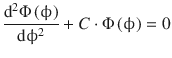
(9.21)

and we recognise by comparison with Eq. 9.16, that this can be resolved to:

(9.22)

In analogy to the case of the rigid rotor with space-fixed axis, the system has to be in the same state after each full rotation, and therefore it can be concluded that

(9.23)

which introduces m as a quantum number.

Instead of the inclination function Θ(θ) the function P(cosθ) is used as a substitute and solving the Schrödinger equation yields the requirement

(9.24)

where m and s are two integer numbers that possess a particular relationship. If one introduces

(9.25)

then the following requirements arise from the relationship between m and s:

(9.26)

From these requirements, it is obvious that m can take the following values:

(9.27)

The function P(cosθ) turns out to be dependent on the two variables m and l and is called the associated Legendre function .

When combining the solutions for the azimuth and the inclination function to yield an expression for the wave function Ψ, one obtains:

(9.28)

with the two quantum numbers l and m. The wave functions obtained are known as spherical harmonics.

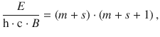
From Eq. 9.24, we can derive the allowed energy states of the rigid rotor with space-free axis (Fig. 9.8):

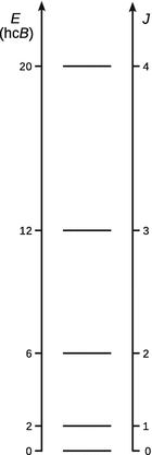
Fig. 9.8

Allowed energy levels for a rigid rotor with free rotation axis

When this model is applied to a molecule, the quantum number J is typically used instead of l:

(9.29)

With setting J = l and Eq. 9.27, it is obvious that for each quantum number l (J), there are (2l + 1) different wavefunctions (one for each value of m) with the same energy. Levels with the same energy are said to be degenerate. For the rigid rotor, the degeneracy of each level is thus (2J + 1).