Physical Chemistry Essentials - Hofmann A. 2018
Quantum Theory of Atoms
10.1 The Hydrogen Atom
In the previous chapter, we familiarised ourselves with various applications of the Schrödinger equation, and can now discuss the hydrogen atom from a quantum mechanical view.
The hydrogen atom constitutes the simplest atomic constellation, comprising a proton and an electron. The potential energy of this system is of electrostatic nature and therefore given by the Coulomb attraction
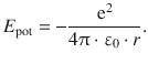
The Schrödinger equation is thus
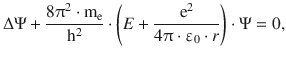
(10.1)
where Δ is the Laplace operator as introduced in Sect. 8.3.1. Since the electrostatic potential takes the form of a spherical potential, it will prove convenient to use the spherical coordinates, so the wave function Ψ depends on r, θ, ϕ: Ψ(r,θ,ϕ). In order to solve the Schrödinger equation, the wave function is separated into three functions, each of which depends on one of the three spherical coordinates
![]()
(10.2)
i.e. a radial function R(r), an inclination function Θ(θ) and an azimuth function Φ(ϕ). The function Y(θ,ϕ) combines the azimuth and inclination functions and resolves to the spherical harmonics we have already introduced when solving the Schrödinger equation for the rigid rotor with space-free axis:
![]()
(9.28)
with the quantum numbers
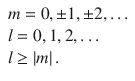
(10.3)
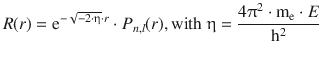
For the radial function R(r), one finds the solution
![]()
(10.4)
where P n, l(r) is a potential development series, and dependent on the quantum numbers
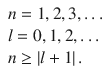
(10.5)
For convenience, the parameter η has been introduced in the exponential function of Eq. 10.4; it is defined as
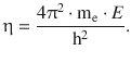
(10.6)
The wave functions that solve the Schrödinger equation for the hydrogen atom are thus functions
![]()
(10.7)
that depend on the three quantum numbers n, l and m; N is the normalisation factor. From Eqs. 10.3 and 10.5 it becomes obvious, the quantum numbers n, l and m have particular relationships and therefore only select combinations are possible as illustrated in Table 10.1.
Table 10.1
Possible combinations of quantum numbers for the first three principal quantum numbers (n = 1, 2, 3)
n |
1 |
2 |
3 |
|||||||||||
l |
0 |
0 |
1 |
0 |
1 |
2 |
||||||||
m |
0 |
0 |
−1 |
0 |
1 |
0 |
−1 |
0 |
1 |
−2 |
−1 |
0 |
1 |
2 |
Since the wave functions Ψ that describe the atom are dependent on the three quantum numbers (Eq. 10.7), there will be a particular number of different wave functions (called linear independent wave functions). The number of possible wave functions is 1 for n = 1, 4 for n = 2, and 9 for n = 3. Due to the general hierarchy provided by the quantum number n, it is called the principal quantum number. Generally, the number of different (linear independent) wave functions is given by
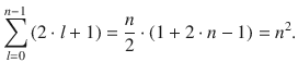
(10.8)
Like in the discussion of the rigid rotor and the harmonic oscillator, the allowed energy levels of the hydrogen atom are not continuous but discrete, and are obtained by considering particular requirements when solving the Schrödinger equation such that the solutions are physically sensible. The allowed energy states ( eigenvalues) of the hydrogen atom are obtained as
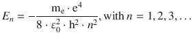
(10.9)
As with previously discussed models, we find that the allowed energy levels of the hydrogen atom vary with a quantum number—specifically the principal quantum number n—and thus there are n different allowed energy levels. At the same time, we derived above (Eq. 10.8) that there are n 2 different wave functions, i.e. measurable different states. The energy levels are therefore said to be degenerate.
Multiple states of a quantum mechanical system are degenerate if they possess the same energy value. Vice versa, an energy level is degenerate, if it corresponds to multiple different measurable states.
The wave functions solving the Schrödinger equation are called eigenfunctions. In the discussion above, we found that those wave functions are best separated into a function depending on the radial (r) and another function depending on the angular spherical coordinates (θ, ϕ). Since it is also necessary to normalise the wave function, a normalisation factor N became a third component; thus:
![]()
(10.10)
In the following sections, we will have a closer look at the radial eigenfunction as well as the spherical harmonics, and then compose the normalised eigenfunctions.
10.1.1 The Radial Eigenfunctions of the Hydrogen Atom
In the previous section, we introduced the solution for the radial function of the hydrogen atom as
(10.4)
An explicit calculation of the exponent in Eq. 10.4 thus yields:
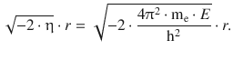
The allowed energy levels are given by Eq. 10.9; therefore:
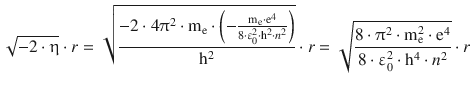
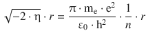
Comparison with Eq. 8.22 shows that the first factor in above equation is the reciprocal of the radius of the first orbit in the atomic model by Bohr:
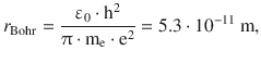
and thus allows us to measure the radius of the electron in multiples of the Bohr radius:
![]() , yielding
, yielding ![]() , and therefore:
, and therefore:
![]()
(10.11)
Notably, the radial eigenfunction described in above Eq. 10.11 is not yet normalised. Table 10.2 summarises explicit normalised radial eigenfunctions for the hydrogen atom; Figure 10.1 illustrates these functions graphically.
Table 10.2
Normalised radial eigenfunctions of the hydrogen atom for n = 1, 2, 3
|
n |
l |
R n,l |
No of radial nodes n−l−1 |
1 |
0 |
R 1, 0 = 2 ⋅ e−ρ |
0 |
2 |
0 |
|
1 |
2 |
1 |
|
0 |
3 |
0 |
|
2 |
3 |
1 |
|
1 |
3 |
2 |
|
0 |
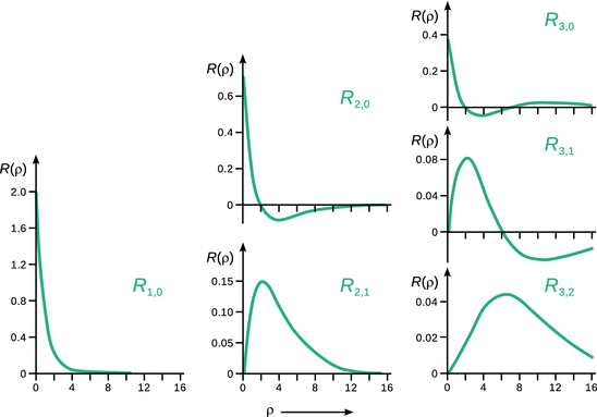
Fig. 10.1
Graphical illustration of normalised radial eigenfunctions of the hydrogen atom for n = 1, 2, 3
Notably, the radial eigenfunction R only depends on the quantum numbers n and l, but not m. From Fig. 10.1, it is obvious that the number of zero-crossings of R increases with n, but decreases with l:
![]()
(10.12)
We have previously introduced for the wave function that the squared function is a probability density to find the particle in particular spatial locations. The same concept applies to the radial eigenfunction, where R 2 describes the probability density to find an electron along a beam originating in the nucleus.
When asking the question of the actual probability to find the electron at a particular distance from the nucleus, e.g. between ρ and (ρ + dρ), the function R(ρ)2 needs to be integrated. For spherical symmetry, the volume of the spherical shell described by ρ and (ρ + dρ) is (4π·ρ2·dρ), which yields for the radial probability distribution
![]()
The plotted probability distribution functions in Fig. 10.2 indicates that for the lowest possible principal quantum number n = 1, the highest probability to find the electron is at the distance of ρ = 1, i.e. r = r Bohr. In this case, we see that the electron can be found in a spherical space around the nucleus, most likely at distance r Bohr. However, the electron does not have a well-defined position and the space where the electron can be found certainly has no sharp boundary. The probability distribution decreases rapidly with increasing distance and anneals to zero at large distances.
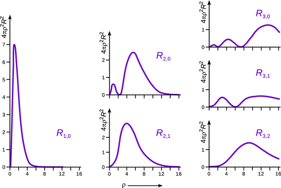
Fig. 10.2
Radial probability distribution functions of the hydrogen atom for n = 1, 2, 3
For the case (n = 1, l = 0) in Fig. 10.2, we see that there are two maxima in the probability density function. Furthermore, there is a region where the probability to find the electron is zero. This region corresponds to the zero-crossing of the radial wave function R(ρ) in Fig. 10.1 and is called a ( radial) node. We can imagine this case as two concentric spheres with a node in between, which takes the shape of a spherical shell.
10.1.2 The Spherical Harmonics of the Hydrogen Atom
When solving the Schrödinger equation for the hydrogen atom, we obtained the spherical harmonics component as
![]()
(9.28)
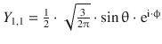
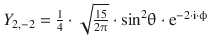
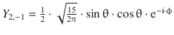
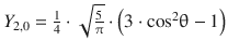
Notably, these functions are not yet normalised and thus need to be multiplied with normalisation factors. The first nine normalised functions are summarised in Table 10.3.
Table 10.3
The normalised spherical harmonics of the hydrogen atom for l = 0, 1, 2
l |
m |
Y l,m |
Number of angular nodes l |
0 |
0 |
|
0 |
1 |
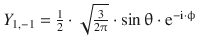
−1 |
|
1 |
1 |
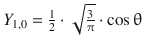
0 |
|
1 |
1 |
1 |
|
1 |
2 |
−2 |
|
2 |
2 |
−1 |
|
2 |
2 |
0 |
|
2 |
2 |
1 |
|
2 |
2 |
2 |
|
2 |

In contrast to the radial eigenfunctions, which depend on only one variable (r or ρ), the spherical harmonics Y possesses two variables, the azimuth angle ϕ and the inclination angle θ. Illustration of the spherical harmonics therefore requires three dimensions. However, from Table 10.3, we learn that for (l = 0, m = 0), the spherical harmonics is independent of both ϕ and θ; it has a constant value of ![]() . Geometrically, this describes a sphere around the origin with a radius of
. Geometrically, this describes a sphere around the origin with a radius of ![]() (see Fig. 10.3 left panel).
(see Fig. 10.3 left panel).
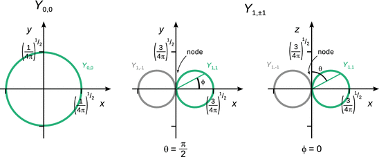
Fig. 10.3
The spherical harmonics functions (angular eigenfunctions) Y 0,0 (left) and Y 1,±1 (centre and right) of the hydrogen atom
The construction of the spherical harmonics for (l = 1, m = ±1) is illustrated in Fig. 10.3 for a particular angle θ (centre panel) and a particular angle ϕ (right panel). The plots show the value of the function Y 1,1 and Y 1,−1 in dependence of the angles ϕ (centre panel) and q (right panel).
As before when discussing the general wave functions Ψ and the radial eigenfunctions R, we are next interested in the probability density which informs about the probability to find the particle in a particular location. For the spherical harmonics Y, the probability distribution is given (similar to Ψ and R) by the squared function, Y 2. (see Fig. 10.4).
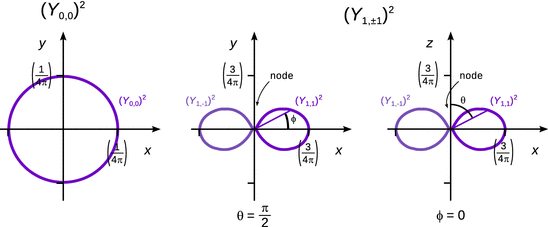
Fig. 10.4
The angular probability distribution functions (Y 0,0)2 (left) and (Y 1,±1)2 (centre and right) of the hydrogen atom
Like with the radial eigenfunctions, we also find for the spherical harmonics that there are areas in which the function Y is zero. In the probability density Y 2, the values in these areas remain zero, thus giving rise to the ( angular) nodes, i.e. areas in which the probability to find the electron is zero. From Table 10.3 it is obvious that the number of angular nodes is given by the quantum number l:
![]()
(10.13)
10.1.3 The Normalised Eigenfunctions of the Hydrogen Atom
Solving the Schrödinger equation for the hydrogen atom led us to the wave functions given in Eq. 10.10, which represent the normalised eigenfunctions of the hydrogen atom.
In a process called separation of variables, we have found solutions for the radial (Sect. 10.1.1) as well as the angular component (Sect. 10.1.2) of those eigenfunctions. Now, we need to combine both of those components, R and Y, and determine the final normalising factor N to obtain the normalised eigenfunctions.
Additionally, since the final wave functions for m ≠ 0 are complex (i.e. contain the number i), linear combinations of the corresponding +m and −m wave functions are generated, which leads to real eigenfunctions (i.e. not containing the number i). For example, the p x and p y orbitals are formed by linear combinations of p +1 and p −1. In contrast, the p z orbital is the same as p 0.
The results are summarised in Table 10.4 and show that the state of the electron is characterised by three quantum numbers:
✵ the principal quantum number n = 1, 2, 3, …
✵ the quantum number l = 0, 1, 2, …
✵ the quantum number m = 0, ±1, ±2, …
Table 10.4
The real eigenfunctions of the hydrogen atom for the principal quantum number n = 1, 2, 3
|
Symbol |
n |
l |
m |
N |
R(r) |
Y(θ,ϕ) |
Radial nodes |
Angular nodes |
1s |
1 |
0 |
0 |
|
e−ρ |
1 |
0 |
0 |
2s |
2 |
0 |
0 |
|
|
1 |
1 |
0 |
2p z |
2 |
1 |
0 |
|
|
cos θ |
0 |
1 |
2p x |
2 |
1 |
±1 |
|
|
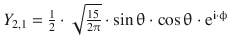
sin θ · cos ϕ |
0 |
1 |
2p y |
2 |
1 |
±1 |
|
|
sin θ · sin ϕ |
0 |
1 |
3s |
3 |
0 |
0 |
|
|
1 |
2 |
0 |
3p z |
3 |
1 |
0 |
|
|
cos θ |
1 |
1 |
3p x |
3 |
1 |
±1 |
|
|
sin θ · cos ϕ |
1 |
1 |
3p y |
3 |
1 |
±1 |
|
|
sin θ · sin ϕ |
1 |
1 |
|
3 |
2 |
0 |
|
|
3 · cos2 θ − 1 |
0 |
2 |
3d xz |
3 |
2 |
±1 |
|
|
sin θ · cos θ · cos ϕ |
0 |
2 |
3d yz |
3 |
2 |
±1 |
|
|
sin θ · cos θ · sin ϕ |
0 |
2 |
|
3 |
2 |
±2 |
|
|
sin2 θ · (sin 2·ϕ) |
0 |
2 |
3d xy |
3 |
2 |
±2 |
|
|
sin2 θ · (sin 2·ϕ) |
0 |
2 |
In addition to the numerical description of electron states by the above quantum numbers, a further nomenclature system ascribes letters to the various different states. The principal energy level (quantum number n) is thought of as a shell in which the electrons orbit; the individual shells are often (especially when referring to X-ray processes) given the letters K, L, M, etc. The quantum number l describes the subshells, denoted by the letters s, p, d, etc (see Table 10.5). The subshells, in turn, comprise of the individual atomic orbitals. As shown in Table 10.4, particular subshells are most commonly denoted by combining the numerical value of the principal quantum number with the letter describing the subshell. The characteristic director of the individual atomic orbital is then added as a subscript. For example, 2p x denotes the p orbital (n = 2, l = 1) which primarily extends along the x-axis.
Table 10.5
Shell and atomic orbital nomenclature
|
Quantum number n |
Shell |
Quantum number l |
Atomic orbital |
1 |
K |
0 |
s |
2 |
L |
1 |
p |
3 |
M |
2 |
d |
4 |
N |
3 |
f |
5 |
O |
4 |
g |
6 |
P |
5 |
h |
7 |
Q |
6 |
i |
7 |
k |
In order to describe the final eigenfunctions, we now need to combine the radial and the angular components. It rapidly becomes clear that this is best done with three-dimensional shapes, since the spherical harmonics depend on two angles, ϕ and θ. The radial eigenfunction provides a measure for how far away from the atomic nucleus an orbital extends, but its nodes might also call for regions in which the electron cannot exist. The angular eigenfunction provides the overall shape information. As illustrated in Fig. 10.5, one might think of atomic orbitals as a sphere, from which particular regions—defined by the nodes—are cut off.
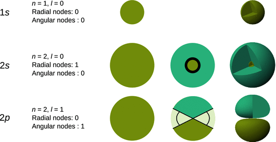
Fig. 10.5
Conceptual construction of atomic orbitals (final eigenfunctions Ψ) from the radial eigenfunction R (sphere), consideration of radial nodes, and application of angular nodes provided by the spherical harmonics (angular eigenfunctions Y). The three-dimensional graphs in the last panel are shown with cut-away wedges to reveal the interior of the functions. The colours indicate positive (blue) and negative (green) values of the wave function Ψ
In the three-dimensional graphs of the final eigenfunctions, the areas where the wave functions assume positive and negative values (phase of the wave function) are typically mapped in different colours (see Fig. 10.5).
The real eigenfunctions, i.e. atomic orbitals, are summarised in Table 10.4 for the principal quantum numbers n = 1, 2, 3. The three-dimensional graphs of these orbitals are shown in Fig. 10.6. The s orbitals (l = 0) possess an overall spherical shape and are nested shells for n > 1. The p orbitals (l = 1) for n = 2 consist of two ellipsoids arranged either along the x-, y- or z-axis. This make-up is very similar for the p orbitals in the shell n = 3, however, an additional radial node leads to four final ellipsoids arranged along the major axis of extension. The shell n = 3 is the first shell with d orbitals, four of which appear very similar and take the form of four drop-like lobes arranged orthogonally around the central nucleus. The centres of all four lobes lie in one plane. These planes are the xy-, xz-, and yz-planes, where the lobes are located between the pairs of the cartesian coordinate system; one of these orbitals has the centres along the x- and y-axes. The fifth d orbital consists of a torus with two pear-shaped lobes placed symmetrically on the z-axis.
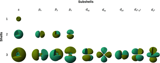
Fig. 10.6
Three-dimensional graphs of the atomic orbitals for the principal quantum numbers n = 1, 2, 3 as summarised in Table 10.4. The atomic orbitals are shown with cut-away wedges. The colours indicate positive (blue) and negative (green) values of the wave function Ψ
It is important to remember that the graphically depictions in Fig. 10.6 are the wave functions Ψ of the individual atomic orbitals. The probability to find the electron within the orbital is given by |Ψ|2, which is a probability density function. Therefore, the shapes depicting the probability is different from those that illustrate Ψ; with exception of the s orbitals, all other orbitals become more prolate when considering |Ψ|2. Also, due to the square operation, there is no longer a difference between positive and negative regions in the orbitals, thus making the probability density functions uniformly positive.