Physical Chemistry Essentials - Hofmann A. 2018
Physico-chemical Data and Resources
1.4 Summary of Important Formulae and Equations
Table 1.10
Important formulae and equations
|
Thermodynamics |
|
|
Boyle’s law The pressure exerted by an ideal gas is inversely proportional to the volume it occupies if the temperature and amount of gas remain unchanged within a closed system. |
V ∼ T |
Charles’ law Gases tend to expand when heated; at constant pressure, the volume is directly proportional to the temperature. |
p ∼ T |
Gay-Lussac’s law If mass and volume of a gas are held constant, the pressure exerted by the gas increases directly proportional to the temperature. |
p ⋅ V = n ⋅ R ⋅ T |
Ideal gas equation The laws by Boyle, Charles and Gay-Lussac combine to the ideal gas equation. |
p solute = K solute ⋅ x solute |
Henry’s law For solutions at low concentrations, the vapour pressure of the solute is proportional to its mole fraction. |
|
Heat capacity at constant volume. |
|
Variation of the internal energy of an ideal gas with volume at constant pressure. |
|
Heat capacity at constant pressure. |
Ideal gas:
Otherwise:
|
Change of enthalpy of a system with respect to a pressure change in an isothermal process. For an ideal gas, there is no change in enthalpy with pressure if the temperature remains the same. |
C p − C V = n ⋅ R |
Relationship between heat capacities of an ideal gas. |
|
Maxwell relations provide a means to exchange thermodynamic functions. |
|
Entropy change of a system with respect to temperature change in an isobaric process. |
|
The pressure dependence of the Gibbs free energy of an isothermal process defines the volume change of the system during that process. |
|
The temperature dependence of the Gibbs free energy of an isobaric process defines the entropy change during that process. |
|
Clapeyron equation Change of vapour pressure of a one-component system with temperature in terms of entropy. |
|
Clausius-Clapeyron equation Change of vapour pressure of a one-component system with temperature in terms of enthalpy. |
|
van’t Hoff equations: reaction isobar and isochore Change of the equilibrium constant of a chemical reaction with temperature. The two equations show the case for isothermal and isobaric, or isothermal and isochoric reactions. |
|
van Laar-Planck isotherm Change of the equilibrium constant of a chemical equilibrium with pressure in terms of the standard reaction volume. |
ΔG = ΔG — + R ⋅ T ⋅ ln K |
Change of the Gibbs free energy of a chemical reaction with equilibrium constant K and standard Gibbs free energy ΔG —. |
|
Colligative properties |
|
Π = i ⋅ c ⋅ R ⋅ T |
Osmotic pressure |
ΔT f = i ⋅ K f ⋅ b |
Freezing point depression |
ΔT b = i ⋅ K b ⋅ b |
Boiling point elevation |
p = p ∗ ⋅ x |
Raoult’s law: vapour pressure depression |
|
Electrochemistry |
|
|
Electrical conductance The conductance increases with the cross-sectional area A and decreases with the length l of the conductor; k is the electrical conductivity. The conductance is the inverse of the resistance R. |
|
Molar conductivity |
m ∼ I ⋅ t = Q |
Faraday’s first law of electrolysis The mass of a substance altered at an electrode during electrolysis is directly proportional to the quantity of electricity transferred at that electrode. |
|
Faraday’s second law of electrolysis For a given quantity of electric charge, the mass of a deposited/generated elementary substance is proportional to the molar mass of that substance divided by the change in oxidation state (i.e. in most cases the charge of the cation in the electrolyte). |
|
Nernst equation Concentration dependence of the Redox potential. |
|
Change of the standard molar Gibbs free energy of an electrochemical process with the standard electrode potential E — and the charge state z. |
|
Henderson-Hasselbalch equation pH of a solution with the buffer system consisting of the weak acid HA and its conjugated base A−. |
|
Kohlrausch’s law The molar conductivity of strong electrolytes increases with decreasing concentrations (valid for generally low concentrations). |
|
Ostwald’s law of dilution The dissociation constant of weak electrolytes is a function of the degree of dissociation α, and with |
Λ0m = ν+ ⋅ λ + + ν‐ ⋅ λ ‐ |
Law of the independent migration of ions The limiting molar conductivity is comprised of the two independent limiting molar conductivities of the anions and cations. |
|
Transport |
|
|
Thermodynamic force A concentration gradient establishes a thermodynamic force F. |
|
Fick’s first law of diffusion Flux of matter is defined by the concentration gradient along x; |
|
Thermal conduction Flux of energy along a temperature gradient; κ is the thermal conductivity. |
|
Flux of momentum When molecules switch from one flow layer to another, their momentum is also migrating; η is the viscosity. |
|
Kinetics |
|
|
Arrhenius equation The rate constants of most reactions depend on the temperature. |
|
The generalised dependency of rate constants on temperature, which applies to all reactions irrespective of their adhering to the Arrhenius relation or not. |
|
Michaelis-Menten enzyme kinetics |
|
Surface adsorption |
|
|
Langmuir adsorption isotherm without dissociation The Langmuir constant K is the ratio of the rate constants for adsorption and desorption: |
|
Langmuir adsorption isotherm with dissociation into two species |
Table 1.11
Kinetic rate laws in their differential and integrated forms, and the derived half lives
|
Order |
Differential form |
Integrated form |
Half life |
0 |
|
c(A) = − νA ⋅ k ⋅ t + c 0(A) |
|
1 |
|
− ln c(A) = νA ⋅ k ⋅ t − ln c 0(A) |
|
2 |
|
|
|
3 |
|
|
|
Table 1.12
Interactions between molecules. α: polarisability; ε0: vacuum permittivity; I: first ionisation potential; μ: dipole moment; r: distance between the two atoms/molecules
|
Interaction |
Potential energy |
Explanation |
Order of magnitude (kJ mol−1) |
Covalent bond |
|V| = 200—800 |
||
Coulomb interaction |
|
Interaction between two ions |
|V| = 40—400 |
Ion-dipole interaction |
|
Interaction between ion and permanent dipole |
|V| = 4—40 |
Keesom interaction |
|
Interaction between two permanent dipoles |
|V| = 0.4—4 |
Ion-induced dipole interaction |
|
Interaction between ion and induced dipole |
|V| = 0.4—4 |
Debye force |
|
Interaction between permanent dipole and induced dipole |
|V| = 0.4—4 |
London dispersion force |
|
Interaction between temporary dipole and induced dipole |
|V| < 0.4 |
|
|V| < 0.4 |
||
Hydrogen bond |
|V| = 4—40 |
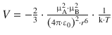
Table 1.13
Interactions of electromagnetic radiation with matter
|
Model/Transition |
Energy |
Selection criteria |
|
Nuclear magnetic resonance |
|
||
Electron spin resonance |
|
Δm s = ±1; Δm I = 0 |
|
Rigid rotor with space-free axis |
E(J) = h ⋅ c ⋅ B ⋅ J ⋅ (J + 1) |
ΔJ = ±1 |
|
Harmonic oscillator |
|
Δv = ±1 |
|
Anharmonic oscillator |
|
Δv = ±1, ±2, ±3, … |
|
Rota-vibrational absorption (Infrared spectroscopy) |
E = E(J) + E(v) |
Δv = ±1 (±2, ±3, …); ΔJ = ±1 |
Singlet molecules |
Δv = ±1 (±2, ±3, …); ΔJ = 0, ±1 |
Non-singlet molecules |
||
Rota-vibrational emission (Raman spectroscopy) |
E = E(J) + E(v) |
Δv = ±1; ΔJ = 0, ±2 |
|
Electronic absorption (UV/Vis spectroscopy) |
E = E(J) + E(v) + E electr |
M = 2 ⋅ S + 1 = const. ⇔ ΔS = 0 |
|
Electronic emission (Fluorescence) |
E = E(J) + E(v) + E electr |
M = const. ⇔ ΔS = 0 |
|
Electronic emission (Phosphorescence) |
E = E(J) + E(v) + E electr |
M ≠ const. ⇔ ΔS ≠ 0 |
|
Optical spectra of atoms |
E = E electr |
Δl = ±1, Δj = 0, ±1 |
Alkali metals |
ΔJ = 0, ±1 |
Multi-electron atoms |
||
Nuclear resonance |
E 2 < 2 ⋅ m ⋅ c2 ⋅ kB ⋅ Θ |
||
X-ray spectra of atoms |
E = E electr |
Δl = ±1, Δj = 0, ±1 |
|
Auger electron spectra |
|
none |
|