Physical Chemistry Essentials - Hofmann A. 2018

The Chemical Bond
11.3 The Covalent Bond

The occurrence of ionic bonds appears as a fairly straightforward phenomenon, since we can easily appreciate its coming-about due to the attraction between two particles of opposite charge. A more complex situation arises when bonds occur between rather similar atoms, i.e. such that exhibit rather small differences in their electronegativity values. Obviously, the formation of particular molecules must result in stable arrangements, meaning that these molecules correspond to a minimum in the overall energy function.

As we have previously seen, even in the case of multi-electron atoms, it is not possible to find an exact solution of the Schrödinger equation. The same problem arises when one considers molecules which comprise of multiple atoms and thus many electrons. Different ways of approximation of such more complex systems have been developed, including the valence bond (VB) method and the molecular orbital (MO) method.

The molecular orbital method, introduced by Friedrich Hund and Robert Mulliken in 1928, considers the nuclear scaffold of a molecule (e.g. the two nuclei of a di-atomic molecule) with varying distances. First, the molecular orbitals are determined; these orbitals localise to multiple atoms (i.e. they are poly-centric), as opposed to the atomic orbitals which localise to just one atom. Then, the molecular orbitals are filled with electrons according to the Aufbau principle as well as the Pauli principle and Hund rules.

11.3.1 The Born-Oppenheimer Approximation

Since atoms comprise of the atomic nucleus as well as electrons, the kinetic energies of both nuclei and electrons need to be considered in a rigorous treatment of energies in a molecule. The Born-Oppenheimer approximation poses that the heavier nuclei remain static at time scales during which the electrons are in movement (see also Franck-Condon principle, Sect. 13.4.1). In other words, this approximation allows separation of the motion of electrons from that of atomic nuclei. In mathematical terms, the wave function of a molecule can thus be thought of as being composed of an electronic and a nuclear function:

(11.11)

At the time scale of electron motion, the atomic nuclei only affect electrons by an electrostatic potential.

11.3.2 Linear Combination of Atomic Orbitals

If we consider a di-atomic molecule consisting of atoms 1 and 2, electrons travel on paths that wrap around both atoms. However, if they are spatially closer to atom 1, they will experience mainly the forces by the nucleus of atom 1 as well as the electrons in its vicinity. The forces originating from the nucleus and electrons of atom 2 are comparably small, due to atom 2 being located further away. The situation electrons find around atom 1 will therefore be similar (but not the same) as if they were part of an isolated atom 1 that is not part of a molecule. The same argument can be made for the situation around atom 2.

It is thus conceivable that the molecular orbital Ψ will have strong characteristics of the individual atomic orbitals Ψ₁ and Ψ₂ in vicinity of either atom 1 or atom 2. Mathematically, this can be modelled by a linear combination of the individual atomic orbitals Ψ₁ and Ψ₂ which constitute the molecular orbital Ψ. The contributions of the individual atomic orbitals—which are now called base functions—don’t have to be the same and are thus expressed in the general form by weighting factors (c ₁, c ₂):

(11.12)

This approach is called the linear combination of atomic orbitals ( LCAO) and can alternatively be formulated as:

(11.13)

where λ is a measure of the polarity of the molecular orbital.

Conceptually the LCAO describes an interference of the two base functions Ψ₁ and Ψ₂. Keeping in mind that the base functions are indeed wave functions, we remember from Sect. 8.1.2 that waves can interfere in a constructive and a destructive manner. In a similar fashion we need to consider a two types of interactions between the base functions; they can either add or subtract, giving rise to two different molecular orbitals, a bonding one Ψ and an anti-bonding one Ψ^*:

As an example, we consider the formation of the hydrogen molecule H₂. The 1s orbitals of each of the individual H atoms combine according to the linear combination of atomic orbitals to yield two molecular orbitals, the σ and the σ^* orbital (Fig. 11.3). Since the σ orbital shows build-up of electron density in the space between two the atomic nuclei, it is called a bonding orbital, since its population with electrons keeps the two atomic nuclei together. In contrast, the σ^* orbital shows low electron density between the two nuclei, hence its population with electrons would lead be destabilising for the assembly of the two atoms; it is called anti-bonding orbital.

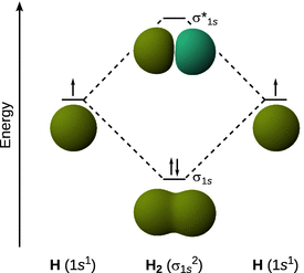
Fig. 11.3

Linear combination of the two 1s orbitals in hydrogen leads to bonding and anti-bonding molecular orbitals of H₂

When considering linear combinations of the p orbitals of two atoms engaging in an interaction, it becomes obvious that there are two types of overlap (Fig. 11.4): In one case, the p orbitals extending along the inter-nuclear axis can overlap and this gives rise to electron density between the two atoms along the inter-nuclear axis. If we think of the inter-nuclear distance as a rotation axis, we appreciate that the resulting orbital has rotational symmetry, just like the σ _s orbital. This type of interaction therefore results in a σ _p and a σ^* _p orbital.

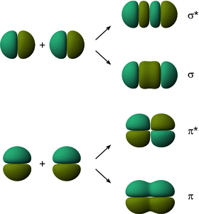
Fig. 11.4

The interaction of two p orbitals can result in formation of either σ/σ^* or π/π^* molecular orbitals

The other two p orbitals have their lobes extending either above/below or in front/behind of the internuclear axis. Overlap of those p orbitals therefore leads to electron density between the two atoms above/below or in front/behind of the inter-nuclear axis. Such orbitals are called π orbitals. As before, constructive and destructive interference is possible, giving rise to two molecular orbitals upon interaction, π and π^*. Notably, the π/π^* orbitals do not possess rotational symmetry, as the sign of those orbitals changes when rotating 180° around the inter-nuclear axis. The relative order of σ- and π orbitals arising from linear combination of 2p orbitals is illustrated in Fig. 11.5.

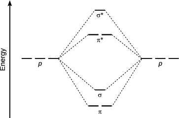
Fig. 11.5

Energy diagram for linear combination of the p orbitals in the second period

Generally, when choosing atomic orbitals for linear combination, three pre-requisites need to be fulfilled:

✵ The energies of the two atomic orbitals need to be at a comparable level.

✵ Both atomic orbitals need to be able to produce sufficient overlap.

✵ The two atomic orbitals need to have the same symmetry with respect to the inter-atomic axis.

11.3.3 Bond Order

We have mentioned earlier that the molecular orbitals are populated with electrons according to the Aufbau principle. Of course, just as in the case of atomic orbitals, the Aufbau principle requires knowledge of the relative energetic levels of the individual molecular orbitals, so that we fill the different orbitals from the bottom to the top. As illustrated for O₂ in Fig. 11.6, this requires that anti-bonding orbitals are populated and we remember that electrons in anti-bonding orbitals result in destabilisation of the bond between two atoms.

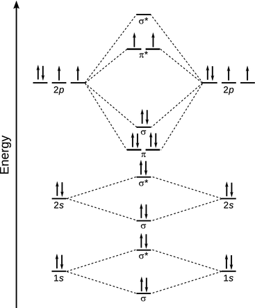
Fig. 11.6

MO scheme for oxygen (O₂)

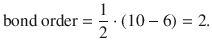
In order to obtain an overall measure of the strength of a bond, the bond order is defined as:

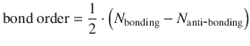
(11.14)

where N _bonding is the number of electrons in bonding and N _anti-bonding the number of electrons in anti-bonding orbitals. For the O₂ molecule (see Fig. 11.6), the border is calculated as per:

11.3.4 Magnetic Properties of Diatomic Molecules

The molecular orbital scheme for oxygen highlights that the O₂ molecule has two unpaired electrons. Because unpaired electrons can orient in either direction, they exhibit magnetic moments that can align with an external magnetic field; such molecules are called paramagnetic. In contrast, molecules that do not possess unpaired electrons are called diamagnetic; they possess no net magnetic moment and are thus not attracted into a magnetic field. Indeed, diamagnetic materials exhibit a weak repulsion to external magnetic fields.

The prediction of the magnetic properties of molecules is a major advantage of molecular orbital theory as compared to the concept of Lewis structures. The concept of Lewis structures, introduced by Gilbert N. Lewis in 1916 (Lewis 1916) for covalently bonded molecules, predicts the bonding between and lone pair electrons of atoms in molecules based on the number of electrons in their outermost shell (the valence shell). For the O₂ molecule, the Lewis structure does not inform about the presence of unpaired electrons (and hence paramagnetism).

Table 11.2 summarises properties of select diatomic gases. Importantly, the bond order and electron configuration determined by the molecular orbital theory correctly predicts the magnetic properties and even the fact that some diatomic molecules (such as for example He₂, Ne₂) do not exist, since their bond order is zero.

Table 11.2

Properties of select diatomic gases. The magnetic properties and bond order are predicted by molecular orbital theory. The experimental values of bond lengths and bond energies reflect the predicted bond order

11.3.5 Dipole Moment

The considerations in the previous chapters assumed that the linear combination of atomic orbitals occurs between two atoms of the same element, which results in formation of homonuclear di-atomic molecules. In the illustrations (Figs. 11.3, 11.5, and 11.6), this manifests itself in the fact that the two interacting atomic orbitals possess the same energy. Moreover, at the level of the quantum mechanical wave function, this results in equality of the two coefficients c ₁ and c ₂ (Eq. 11.12) or λ = ±1 (Eq. 11.13).

Whereas the same methodology can be applied to hetero-nuclear di-atomic molecules, we appreciate that the two atoms no longer belong to the same element, hence the energies of the interacting atomic orbitals are no longer equal. Similarly, the weighting coefficients c ₁ and c ₂ are not the same, and λ ≠ ±1.

As mentioned in Sect. 11.3.2, the coefficient λ is a measure of the polarity of the molecular orbital, and if its value deviates from 1, the bond possesses a permanent electric dipole momentum (i.e. a bond moment). This is a result of one atom in the molecule attracting electrons more strongly than the other, leading to a formal partial negative charge on one atom and a formal positive charge on the other. In general, a dipole moment μ arises from a charge separation in space, and is thus defined as

(11.15)

where Q is the separated charge (e.g. 1 · e = 1.602 · 10⁻¹⁹ C) and r the distance between the positive and negative centres. Since such separations happen at the scale of a chemical bond, the dipole moment is measured in multiples of 3.338 · 10⁻³⁰ C m which is called the debye:

and leads to the dipole moment for the charge separation due to one electron displaced by 1 Å = 0.1 nm = 10⁻¹⁰ m of

When assessing the overall dipole moment of a molecule, one considers the individual bond moments as vectors (i.e. they have a value/length and a direction) and estimates the overall dipole moment by vector addition.

Table 11.3 compares bond moments of some select heteronuclear bonds with the electronegativity difference between the two atoms. If the dipole moment in a bond becomes larger, this results in the bond adopting more and more ionic character.

Table 11.3

Examples of bond moments and electronegativity difference of the constituting atoms

Dipole Moment of Ionic Compounds

The electronegativity difference between Na and Cl of 2.1 suggests that NaCl forms an ionic bond. If the bonding in crystalline NaCl was 100% ionic, the charge on the sodium atom was +1·e, and the charge on the chlorine −1·e. With an inter-nuclear distance of 2.36 Å, this results in a dipole moment of μ = 11.34 D. The experimental value of the dipole moment can be obtained by microwave spectroscopy and yields μ = 9.001 D. The ratio of the experimental and theoretical dipole moments

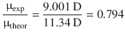
indicates that the bonding between sodium and chlorine in the ionic solid is ~80% ionic.