Physical Chemistry Essentials - Hofmann A. 2018

Thermodynamics
2.1 Motivation, Revision and Introduction of Basic Concepts

The description of macroscopic phenomena in the area of chemistry, biology, physics and geology is of eminent importance to develop an appreciation and understanding of the molecular processes that give rise to these phenomena. Thermodynamics is a systematic theory that is applicable and valid in a truly general fashion. As such, the knowledge of thermodynamic concepts is a pre-requisite for many neighbouring disciplines, such as materials science, environmental science, biochemistry, forensics, etc.

In particular, thermodynamics is concerned with

✵ how the macroscopic world behaves

✵ how energy is transferred

✵ how and under which conditions equilibrium is achieved

✵ how and into which direction processes develop.

Despite the fact that the complex looking formulae may be obtained and dealt with at times, the study of thermodynamics is constantly connected to observations made in the real macroscopic world. The laws of thermodynamics are a prime example of how the theory is connected with real world experiences.

The types of question we might want to answer may include:

✵ If we have a fluid in a sealed container, how will the pressure in the container likely change with temperature?

✵ Is the solubility of a compound likely to increase or decrease with temperature?

Application of thermodynamic concepts will allow us to answer such questions qualitatively, but, more importantly, we will also be able to derive quantitative answers. It is thus necessary to use some algebra and calculus (see Appendix A).

2.1.1 Fundamental Terms and Concepts

It seems appropriate to start with the introduction and revision of vocabulary frequently used in thermodynamics. Many fundamental terms and concepts are typically introduced in entry-level chemistry courses, and should thus already be familiar (Table 2.1).

Table 2.1

Summary of fundamental physico-chemical terms and concepts

In the following Sects. (2.1.2—2.1.13), we will expand these fundamental concepts so that we can start to explore various thermodynamic concepts in more detail.

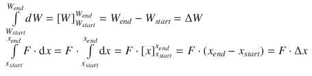
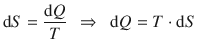
All physical measurements are about differences, absolute values of quantities can not be determined. Therefore, when describing quantities such as functions (e.g. energy, entropy) and observables (e.g. temperature, pressure), they are typically characterised by comparing two different states, such as for example the energy difference between two different states that possess different temperatures. When such differences are observed macroscopically (i.e. in a typical bench-top experiment), these differences are denoted with a capital Greek delta (Δ). In other words, the Δ describes the difference between two reasonably spaced discrete points. When an infinitesimally small difference between two very close points is addressed, the lower case Greek δ is used instead. For quantities that can be expressed as continuous mathematical functions, the ’δ’ becomes a ’d’ to indicate the differential of that quantity. The differential of a quantity with respect to another can be envisaged as the slope of the curve in a plot of the two quantities (see Fig. 2.1).

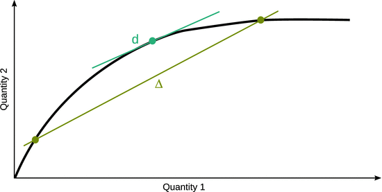
Fig. 2.1

Comparison of the macroscopic difference Δ between two discrete points and the differential as a special case of difference where two neighbouring points merged into one

A basic introduction to differentials is given in Appendix A.2. Throughout this text, we will use ’Δ’ to denote a macroscopic difference, and ’δ’ or ’d’ for infinitesimal small differences. Since differentials (’d’) allow application of mathematical formalism and calculus, this will frequently be the notation of choice. It is important to remember, that any differential can be seen as a difference between two states. The macroscopic difference of a function X, ΔX, is linked to the many microscopic differences dX within a range from X _start to X _end by the mathematical process of integration:

System

All scientific study is carried out on a particular system that is the subject of study. A system is the part of the universe that can be conveniently studied with the methods at hand. In many cases, most or all of the properties of the system are under the control of the observer. A system can be as simple as a container filled with water that is placed on a heating plate.

Systems can be subdivided based on their boundaries. It may not always be possible to perfectly reproduce such boundaries in real experiments, but for the development of concepts, idealised versions are required. Typically, three types of systems are considered:

✵ isolated system: can neither exchange energy nor matter with its environment; it thus cannot elicit any changes in the environment nor can it be changed by its environment.

✵ closed system: whereas exchange of energy is allowed between the system and its environment, it is not possible to exchange matter.

✵ open system: the exchange of energy as well as matter is possible, as e.g. between two compartments separated by a semi-permeable membrane.

Equilibrium

A system that has reached equilibrium does not show any macroscopic signs of change, i.e. there is no change of the state of that system.

Intensive and Extensive Parameters

State variables are parameters that describe particular properties or coordinates of a system. They can be classified into two groups:

✵ extensive parameters—depend on the amount of substance present in the system. The value of extensive parameters can be calculated as the sum of the partial values when the system is subdivided into parts.

✵ intensive parameters—do not depend on the amount of substance present in the system. The value of intensive parameters can be measured at any point within the system.

Typically, an intensive parameter can be calculated as the quotient of two extensive parameters.

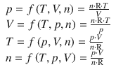
Temperature

Temperature is a measure for the average kinetic energy () of particles in a container:

(2.1)

where k_B is the Boltzmann constant: = 1.380662·10⁻²³ J K⁻¹, and ε_kin is used to indicate the extensive kinetic energy (since it is measured per particle; [ε_kin] = 1 J), as opposed to the intensive quantity E _kin (measured per mol; [E _kin] = 1 J mol⁻¹).

Temperature is an intensive property and therefore does not depend on the amount of substance in the container. The temperature indicates the direction of the flow of energy through a thermally conducting wall. If energy flows from object A to B when they are in contact, then A is defined to possess higher temperature. Thermal equilibrium exists, when no energy flow occurs between objects A and B when they are put into contact by a wall that allows heat to flow.

There are various scales (and thus units) of measurement for temperature (Table 2.2):

Table 2.2

Commonly used temperature scales

The fix points of the Celsius scale are defined as −273.15 °C = 0 K and the triple point of water being at precisely 273.16 K and 0.01 °C (at standard pressure). Thus, the increments on the degree Celsius and kelvin scale are the same, which led to the recommendation that temperature differences on the degree Celsius scale should be expressed in kelvin; for example:

although this rule has been relaxed by IUPAC (Rossini 1968). According to above definition, temperatures on the kelvin and degree Celsius scales can be converted as per

(2.2)

The standard temperature as defined by IUPAC is at

as opposed to the normal temperature of

which is typically used as a reference temperature for many physico-chemical processes and chemical reactions.

Pressure

Pressure is defined as the force divided by the area to which the force is applied

(2.3)

Pressure is an intensive property and thus does not depend on the amount of matter present.

There are various scales (and thus units) of measurement for pressure (Table 2.3):

Table 2.3

Commonly used pressure scales

The IUPAC standard pressure is defined as

(2.4)

The normal pressure (which equals the standard pressure used by the National Institute of Standards and Technology, NIST, USA) refers to atmospheric pressure and is defined as

(2.5)

Mechanical equilibrium exists when a moveable piston between two compartments filled with gases has no tendency to move.

Boiling points depend on the pressure

Since water boils at a temperature of θ_b,normal (H₂O) = 100 °C at normal pressure (p_normal = 1 atm = 1.013 bar), the boiling temperature is less at IUPAC standard pressure (p^— = 1 bar = 0.9869 atm).

Ideal Gas

The behaviour of an ideal gas can be explained by the kinetic gas theory which requires the following assumptions:

✵ the gas is composed of particles whose total volume is negligible compared with the volume of the system

✵ the interactions between particles are negligible

✵ the average kinetic energy is proportional to the temperature

The ideal gas equation constitutes the equation of state for the ideal gas and informs about the physical state of the system for given conditions:

(2.6)

The variables and parameters of the ideal gas equation are (Table 2.4):

Table 2.4

Variables and parameters of the ideal gas equation

Partial Pressure

If a system contains more than one gaseous components, the partial pressure describes the pressure of any particular gas if it would reside there alone, under the same total pressure and temperature. In case of ideal gases, the ideal gas equation is valid for each individual gas with its partial pressure:

(2.7)

Dalton’s law poses that the pressure exerted by a mixture of gases is the sum of the partial pressures of the individual gases:

(2.8)

Example of Dalton’s law

If we have a mixture of O₂ and N₂ in a flask, where the partial pressure of O₂ is p(O₂) = 1 Pa, and the partial pressure of N₂ is p(N₂) = 2 Pa, the total pressure in the flask is

Energy

Energy describes the capacity to do work and thus bring about change. Energy is measured in units of joule: [E] = 1 J.

Work

Is a form of energy and can be classified either as mechanical or electrical work. Mechanical work is defined as the product of a force and the length along which this force is applied:

(2.9)

electrical work is done when a current I flows through an electric resistance R over a particular time t.

(2.10)

Differential expressions

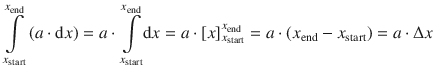
Since energy is all about the potential to change the state of a system, differential expressions are frequently used. The differential expression for mechanical work tells us how much the value of the work changes (dW) when the force F is applied along a particular distance (dx):

Differential expressions need to be integrated in order to obtain a definite value. To integrate this expression, the following integrals need to be resolved:

The value of the work done is thus:

Heat

When energy changes as a result of a temperature difference between the system and its surroundings, we say there is a flow of heat ΔQ. If there is no flow of heat during a process, this is called an adiabatic process. Heat therefore is an energy due to temperature; it is measured in units of joule: [Q] = 1 J. Like work, heat is a path function, i.e. the amount of heat flow depends on the way the change occurs.

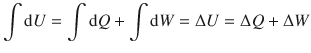
Internal Energy

Internal energy describes the energy possessed by system, in addition to its kinetic and potential energy:

(2.11)

E _kin and E _pot are macroscopic parameters of a system and, in general, can be treated as constant. The internal energy U is an extensive state parameter and depends on the internal state variables V, T and n. If the external state variables E _kin and E _pot are constant, the change in the energy of a system (ΔE) equals the change in the internal energy (ΔU) and comprises of the work done (ΔW) and the exchanged heat (ΔQ):

(2.12)

If we do not change the amount of substance present in the system (i.e. n = const.), the ideal gas equation relates the three state variables p, V and T (and in order to define the state of a system, it is thus sufficient to experimentally restrain two parameters (e.g. V and T), as the third one (here: p) will follow suit. Since for gases, the volume can be controlled rather conveniently, the internal energy U is generally described as a function of V and T. The internal energy is measured in units of joule: [U] = 1 J.

Enthalpy

Whereas the volume of gases can be controlled or changed rather readily in an experimental setting, this is not the case for the condensed phases of liquids and solids. The thermal extension of the volume of solids and liquids can hardly be prevented. From an experimental perspective, it is thus easier to characterise the energy of systems with condensed phases under constant pressure. This is a reasonable criterion, as the ambient pressure can be considered constant for most laboratory experiments. This energy function is the enthalpy H, which is defined as

(2.13)

The enthalpy is measured in units of joule: [H] = 1 J.

Entropy

Entropy describes the dispersion of energy (’disorder’) and is defined as

(2.14)

The entropy is measured in units of joule per kelvin: [S] = 1 J K⁻¹.

Units of measurement

Efforts to standardise the units of measurement started around 1800 with the central idea of choosing a natural constant as reference. This resulted in the metric system whereby the length of 1 m was defined as one 10⁻⁷-th of the length of the quarter meridian of the earth. The current units of measurements (see Table 1.4) are the result of further efforts into that direction and are defined in the International System of Units ( SI) (Bureau international des poids at mesures 2006). In the current system of units, the kilogram is defined by a mass protoype in form of a Pt-Ir cylinder, deposited in the Bureau International des Poids et Mesures (BIPM). By definition, the mass of this protoype is 1 kg, but its real mass has changed over time by contamination; it is estimated to have gained 0.1—0.3 mg as compared to its initial mass. The unit of the molar amount—the mol—is defined via the carbon isotope ¹²C whereby the molar mass of this isotope is set to be 0.012 kg mol⁻¹. Therefore, the definition of the mol depends on the definition of the kilogram.

In the recent past, it has been debated that a more robust referencing is required to become independent of protoypes which change over time (Bureau international des poids at mesures 2013). One of these suggestions proposes that in the new system, the unit of mol shall be linked to an exact numerical value of Avogadro’s constant N_A, which will make it independent of the kilogram (which in turn may be defined via an exact numerical value of Planck’s constant h). Consequently, the unit of 1 mol would be the amount of exactly 6.02214129·10²³ particles (Stohner and Quack 2015). Conceptually, in this new system, the numerical value of N_A would be fixed and thus no longer carry a statistical uncertainty as in the present system (estimated at 5·10⁻⁷). At the same time, the molar mass of ¹²C, which currently is an exact quantity, will become an experimental quantity in the new system and thus be subject to statistical uncertainty. It is estimated that this uncertainty will be at the order of 10⁻⁹ which needs to be set into relation with the uncertainty of general molar masses (approx. 10⁻⁵). One can thus anticipate that there will be no substantial changes of atomic masses in the periodic system if this new system should be instantiated. Nevertheless, the debate about such changes to the SI are ongoing and, at present, subject to further evaluation by the International Union of Pure and Applied Chemistry ( IUPAC) (International Union of Pure and Applied Chemistry 2013).

2.1.2 The 0th Law of Thermodynamics

From the empirical quantity temperature and the equilibrium concept, one can deduce the 0^th law of thermodynamics:

If two systems (A and B) each are in thermal equilibrium with a third system (C), then they are also in equilibrium among each other (i.e. A with B). All three systems share a common property, they have the same temperature.

This law implies that the boundaries of a system may possess thermal conductivity. We consider two compartments of a large container that are separated by a styrofoam (i.e. isolating) wall. If we put hot water into one compartment, and cold water into the other compartment, the two systems will have different heat, and this state will not change. If the styrofoam wall is replaced with a metal foil, there will be a change of the states of both compartments. Heat will flow from the hot to the cold water compartment. The heat flow will cease, when both systems are in thermal equilibrium. At that point, both compartments have the same temperature.

2.1.3 Equations of State

The physical state of a system is described by its physical properties. The parameters describing these properties are called state variables or state functions. State variables are defined in terms of the various properties we can attribute to a substance. For example, the state of a pure gas is specified by giving its volume (measured in liter), the amount (measured in moles), pressure (measured in Pa) and temperature (measured in K).

There will be a relationship between the different state variables, i.e. they are not independent from each other. Such relationships are called equations of state. In the case of a gas, this relationship is given by the ideal gas equation.

(2.6)

It follows from the ideal gas equation that if one specifies three of these four variables, the fourth one will have one discrete value. Each state variable is thus a function of the three others:

Important state variables in thermodynamics are (Table 2.5):

Table 2.5

Important thermodynamic state variables

2.1.4 Energy

Energy describes the capacity of a system to do work. It is a state function and an extensive parameter, since its value depends on the amount of substance. It is measured in units of joule, albeit some reference to the historically used calorie unit may still be found:

There are various types of energies, including:

✵ kinetic energy: (Newtonian mechanics)

✵ potential energy: E _pot = m ⋅ g ⋅ h; g = 9.81 m s⁻² (Newtonian mechanics)

✵ chemical energy: energy present in the bonds between atoms and molecules

✵ thermal energy: due to the vibration and movement of the atoms and molecules in a substance

✵ electric energy: potential difference between two half-cells with electron conducting link

✵ osmotic energy: difference in salt concentration in two half-cells separated by a semi-permeable membrane

Since potential and kinetic energy refer to the position or movement of the system, they are considered external, macroscopic parameters of the system. All other types of energies possessed by the system are combined and constitute its internal energy.

2.1.5 The 1st Law of Thermodynamics

Energy cannot be made or destroyed. Since the internal energy of a system comprises all energy that this system possesses, it follows that any change of the internal energy of a system has to be the result of the work done and the heat transferred:

(2.12)

and as such constitutes the 1^st law of thermodynamics:

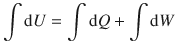
For a closed system with constant external state variables, the internal energy U constitutes an extensive state function whose change dU is composed of the exchanged heat dQ and work dW done on or by the system.

(2.15)

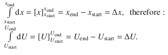
Whereas above the 1st law is defined for the differential change dU, the same is true for the macroscopically measurable change ΔU (see Eq. 2.12), which represents the integrated form of the differential Eq. 2.15.

The integrated form of the differential equation dU = dQ + dW

Differential changes are infinitesimally small changes in variables. Processes that are observed macroscopically have definite start and end points. It is thus necessary to integrate the differential equation.

(2.16)

Integration needs to be carried out with respect to each differential variable. Hence the left side of Eq. 2.16 has one integral (as there is only one differential variable, dU), but the right side has two integrals (one integrating dQ and one integrating dW).

In order to resolve ∫dU, we replace U with x and obtain ∫dx. This function has a known integral (see Appendix A.3.1):

It is immediately obvious, that ∫dQ and ∫dW can be resolved in the same fashion:

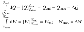
It thus follows:

Note that the 1st law contains one important restraint; it is valid for closed systems which requires that only energy, but no matter can be exchanged. Besides this restriction, the 1st law is generally applicable and in particular applies to reversible as well as irreversible changes of state.

In Sect. 2.1.1, we defined isolated systems by the fact that they cannot exchange any energy with their environment. It follows that the internal energy of an isolated system remains constant, because:

If there is no change in internal energy (ΔU = 0), the internal energy is constant: U = const.

2.1.6 Work

Work is done when an object is moved against an opposing force. This could for example be electrons moving through an electric conductor (electrical work), molecules moving in space under atmospheric pressure (work of expansion/compression). If a system does work of the value ΔW, its internal energy changes by this amount of energy:

(2.12)

The amount of work that a system does, depends on how a particular process occurs. The same final state of the system may be reached by different pathways which require different amounts of work. Therefore, work is a path function.

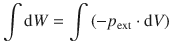
The amount of work to be done for contraction or expansion will depend on the change of the volume of the system (ΔV = V _final − V _initial) and the surrounding restrictions presented by the external pressure p = p _ext. The amount of work done by expansion or contraction can macroscopically be calculated as

(2.17)

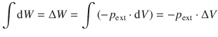
If we consider very small changes, we need to move from the macroscopic difference (Δ) to a differential (d):

(2.18)

The integrated form of the differential equation dW = −p _ext·dV

To initiate integration of this equation, we add the integral sign ∫ to both sides of the equation:

(2.19)

The left side of this equation can be resolved easily by

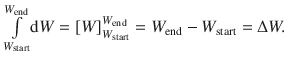
The right side of Eq. 2.19 takes the form of ∫(a ⋅ dx) where a is a constant that does not depend on the differential variable dx. The external pressure is the environmental (ambient) pressure and is not affected by the volume change of the system under study, which is considered negligibly small compared to the earth’s atmosphere. The integral ∫(a ⋅ dx) is resolved as:

and with a = − p _ext, x = V we obtain:

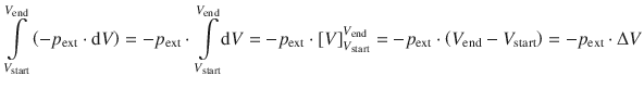
and therefore

There are two interesting cases of expansion/compression work, we should look at in more detail. First, if the external pressure is zero (which is the case in a vacuum), Eq. 2.17 yields:

so there is no work done, despite the fact that the system may expand.

Second, if the external pressure is gradually changed by infinitesimal small amounts so that the internal and external pressures remain equal at all times, the expansion/compression is carried out reversibly. Changes will occur infinitesimally slowly, and the system will be at equilibrium with the surroundings at all times. In that case, the pressure in Eq. 2.18 is no longer constant, but varies with the change in volume: p = p(V). The work done in reversible processes is therefore calculated as per the following integration:

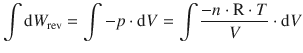
(2.20)

If we consider an ideal gas, we can express the pressure p as a function of the volume V using the ideal gas equation. If we further consider that the reversible volume work is carried out under constant temperature ( isothermal process), then the product n ⋅ R ⋅ T forms a constant that can be taken outside the integral:

The integral is of the form (see Appendix A.3.1). The reversible expansion/compression work thus resolves to:

With the logarithm rule of (Appendix A.1.2), this yields:

(2.21)

Figure 2.2 compares the irreversible (p _ext = const.) and reversible (p _ext is variable) expansion/compression work under isothermal conditions (T = const.). The work is represented by the indicated area under the p-V-curve. From this comparison, it is evident that the magnitude of the work is maximised in a reversible process.

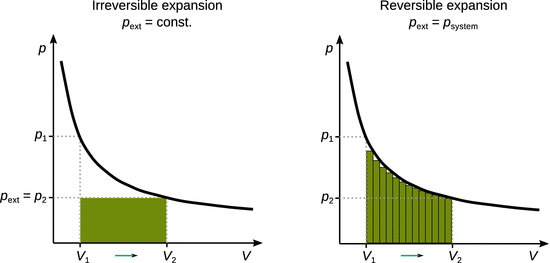
Fig. 2.2

Work done during isothermal irreversible (left) and reversible (right) expansion processes. In irreversible processes, the external pressure is constant and the expansion from V ₁ to V ₂ happens in a single step, resulting in an amount of work indicated by the shaded area. In reversible processes, the external pressure is at all times equal to the pressure of the system (p), and the amount of work done can be estimated by small incremental areas. The total amount of work for the reversible process is larger than that for the irreversible process

2.1.7 Heat Capacity at Constant Volume

The change in the internal energy of a substance when the temperature is raised is described by the heat capacity at constant volume (indicated by the subscript V):

(2.22)

It follows straight from Eq. 2.22 that the internal energy of a system varies linearly with temperature, if the volume remains constant:

(2.23)

If the heat capacity does not change in the temperature range being considered, then one can use Eq. 2.23 to determine the heat capacity C _V by measuring the heat ΔQ _V provided to the system. Since we still require the volume to be constant, the system will not be able to do any expansion/compression work, i.e. ΔW _V = 0:

Experimentally, one can provide a defined amount of heat to a system, for example by electrically heating the system in a bomb and observing the temperature change in the system. The closed bomb case will ensure that the volume remains constant during the process. The bomb will also need to be insulated such that there is no exchange of heat possible with the environment, which is called an adiabatic system. A plot of ΔQ _V versus ΔT will yield a line with the slope C _V . The instrument used for this purpose is an adiabatic bomb calorimeter.

The heat capacity is measured in units of joule per kelvin:

Since the internal energy U is an extensive function, the heat capacity at constant volume is extensive, too. Its value increases with the amount of substance in the system. The corresponding intensive properties of matter are:

✵ molar heat capacity: heat capacity of 1 mol of substance

✵ specific heat: heat capacity of 1 g of substance.

2.1.8 Enthalpy

If we consider an open container filled with liquid water that is being heated, we know from experience that the water will expand its volume as it gets hotter (Fig. 2.3 left). In addition to the heat ΔQ transferred into this system, we further have to consider the volume work ΔW which the system performs as it pushes back the atmosphere. Thus, the change in internal energy ΔU during the heating process is

(2.12)

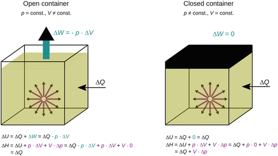
Fig. 2.3

Comparison of the energy changes upon heat transfer into a system residing in either an open or closed container highlights the usefulness of the enthalpy for “everyday experiments”, typically conducted under ambient (i.e. constant) pressure

As the expansion/compression work is a frequently occurring step in many chemical processes, it would help to simplify the description of energy changes of systems, if this work could be accounted for automatically. Therefore, the enthalpy H is defined as

(2.13)

and is measured in units of joule: [H] = 1 J. This quantity takes into account the simultaneous loss (or gain) of energy by expansion/compression, when the energy of the system is changed.

In order to calculate an enthalpy change, we need to differentiate Eq. 2.13:

With the product rule (Appendix A.2.3) for differentiation this yields:

If we assume constant external pressure (p = const.), which is the case for processes carried out under ambient pressure, it follows that dp = 0:

(2.24)

If we again consider the open container with water that is getting heated, we know that this system will expand and thus conduct work against the outside pressure; the internal energy change is thus:

from Eqs. 1.15 and 2.18.

Substituting this expression for dU in Eq. 2.24 yields:

(2.25)

Therefore, the enthalpy change of the system during heat transfer under constant pressure is the same as the transferred heat, if no other work (than expansion/compression) is done.

Reactions or processes that involve solids or liquids and gas/vapour are typically characterised by large changes in volume, i.e. dV is not negligible. However, if a reaction or process involves only liquids and solids, the product p ⋅ V is rather small, therefore H ≈ U. With ΔH = ΔQ ≈ ΔU, the change in internal energy ΔU can be measured by evaluating the heat exchange ΔQ.

Enthalpy change of a closed container with liquid upon heating

We again heat a container filled with liquid, but now require that the container is closed. This means that the volume of the system can not expand during the heating process (Fig. 2.3 right).

Evaluating the change in enthalpy of this system during the heating process, we obtain:

(2.13)

With the product rule (Appendix A.2.3) for differentiation this yields:

Since the container is closed, we know that V = const. and thus dV = 0:

(2.26)

For the internal energy of the closed container, the following change arises:

from Eqs. 2.15 and 2.18

Due to dV = 0 it follows that:

(2.27)

Since the container is closed, the system cannot expand and thus not do any work; the internal energy equals the transferred heat. This delivers the theoretical basis for the adiabatic bomb calorimeter (Sect. 2.1.7), where the heat capacity C _V of a substance can be determined from the linear relationship between transferred heat and temperature, based on the fact that dU = dQ.

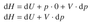
However, for the enthalpy, we obtain the following expression by combining Eqs. 2.26 and 2.27:

(2.28)

The enthalpy change of the closed container thus comprises more than just the amount of heat transferred; the pressure change inside the container further adds to the enthalpy.

Enthalpy is a thermodynamic potential. Potentials cannot be measured in absolute terms; rather, one needs to refer to a defined reference point. Practically, one thus measures only changes in enthalpy, ΔH.

Furthermore, enthalpy is an extensive property, i.e. it depends on the amount of substance in a system. The corresponding intensive property is the molar enthalpy H _m, which is normalised with respect to 1 mol: [H _m] = 1 J mol⁻¹.

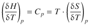
2.1.9 Heat Capacity at Constant Pressure

Like the internal energy, the enthalpy of a system can vary with temperature, and this variation is described by the heat capacity. Whereas the heat capacity derived from the internal energy refers to processes at constant volume (C _V ), the heat capacity derived from the enthalpy refers to processes at constant pressure:

(2.29)

Since enthalpy characterises processes at constant pressure, it can be evaluated by monitoring the change in temperature of a system in cells that are not closed (p = p _ext = const.). This type of analysis is called calorimetry. Whereas differential scanning calorimetry (DSC) evaluates enthalpy changes as a function of temperature (e.g. to determine the heat capacity C _p ), isothermal titration calorimetry (ITC) is used to monitor enthalpy changes due to chemical processes (binding, reactions) at constant temperature.

Relationship between heat capacities for an ideal gas

From the definition of the heat capacity at constant pressure (Eq. 2.29), we obtain by resolving for dH:

From Eq. 2.24 we know that

Therefore, we obtain

Using Eq. 2.22 we can substitute for dU:

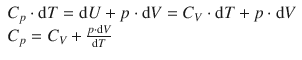
By resolving the ideal gas equation (with the differentials dV and dT)

for , it becomes clear that

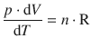
Therefore:

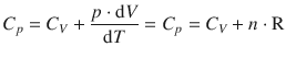
or

2.1.10 Entropy

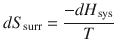
Entropy describes the disorderly dispersal of energy. The change in entropy is related to how much energy is reversibly transferred as heat (see Eq. 2.14). A system that disperses heat into its surroundings without doing any other expansion/contraction work (dW = 0) therefore changes the entropy of the surroundings by:

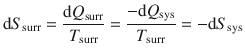
(2.30)

For a process at constant pressure, the enthalpy change in the system dH _sys can be used to determine the entropy change of the surroundings, since we know from Eq. 2.25 that dH = dQ; therefore:

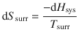
(2.31)

For reversible adiabatic processes, which do not allow the exchange of heat with the environment, it follows from Eq. 2.30 that there is no change in entropy:

(2.32)

Reversible processes refer to processes that occur while the system remains at equilibrium at all times. They are generally hypothetical, unless there is no overall change occurring in the system. An equilibrium can be considered as a state of the system where there is cross-over from the forward to the reverse reaction, both of which occur spontaneously. Obviously, for such processes there will be no change in the entropy:

(2.33)

Important equilibrium process are those of phase transitions, such as a substance boiling at its boiling point. The entropy change during this process is defined by the enthalpy of vapourisation ΔH _vap:

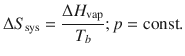
(2.34)

Similarly, the entropy change of a substance freezing at its freezing point is given by:

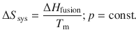
(2.35)

In both Eqs. 2.34 and 2.35, we are using ’Δ’ instead of ’d’ to indicate that these are macroscopically observable changes. As given, both equations are expressions for the entropy change of the system (ΔS _sys) that undergoes the phase transition. One should keep in mind that the entropy change of the system is related to that of the surroundings by:

(2.30)

2.1.11 The 2nd Law of Thermodynamics

Observation of general phenomena tells us that there is a direction associated with all processes, for example a compound dissolving in a solvent or hot coffee getting cold. It then becomes obvious that no process is possible in which the sole result is the absorption of heat from a reservoir and its complete conversion into work; energy is always dissipated. In the example of the hot coffee getting cold, the heat disappearing from the cup does not result in any useful work. It is rather dissipated into the environment and cannot be re-captured.

These concepts are summarised in the 2nd law of thermodynamics:

The entropy of the universe increases in the course of every natural change:

(2.36)

As a consequence, this law predicts what direction a process or reaction will follow. It further produces interesting implications, such as the phenomenon that the direction of a macroscopic process is always the same. The hot coffee gets colder if it is let to stand—it never gets hotter.

Another intriguing aspect of social importance and the way science is communicated is the problem commonly referred to as ’ energy crisis’ which refers to the dwindling energy resources on earth. A critical appraisal of the 1^st law of thermodynamics shows that such concerns are unwarranted. Energy cannot be destroyed, so there is no worry that it would be depleted. Rather, it is the way in which energy is being dispersed that constitutes the problem. By consuming energy, we increase the entropy (i.e. disperse the energy) and thus destroy its availability. In this sense, there is an ’entropy crisis’ rather than an ’energy crisis’.

2.1.12 The 3rd Law of Thermodynamics

A relationship of practical importance for the determination of entropy changes of substances at constant pressure can be derived from

(2.25)

and

(2.30)

The enthalpy change during a process can then be expressed by

(2.37)

whereby the temperature dependence of this process is given by the heat capacity at constant pressure, C _p :

(2.29)

This yields with Eq. 2.37:

(2.38)

and upon integration in the temperature interval from 0 to T _end:

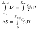
(2.39)

If one knew the entropy of a substance at T = 0 K, it would be possible to determine absolute entropy values. For this reason, Planck postulated that the entropy of a pure, homogeneous phases in internal equilibrium at zero temperature would be zero.

In crystals, which represent pure homogeneous phases, the state of internal equilibrium is attained when there are no defects in the lattice. This postulate is an extension of the Nernst heat theorem:

(2.40)

which states that the entropy of pure substances in their perfect crystalline state at T = 0 tends to zero. This forms the basis of the 3^rd law of thermodynamics:

If the entropy of every element in any crystalline state at T = 0 is set to zero (S ₀ = 0), then all substances have a positive entropy. At T = 0, the entropy of substances in their ideal crystalline states is zero.

Since real crystals of substances are virtually impossible to attain, there is a remaining non-zero entropy of such real systems. A prominent example in this context includes glasses. In substances, where there is a possibility of varying molecular orientation within the crystal lattice (e.g. CO: C─O vs. O─C; N₂O: N─N─O vs. O─N─N), a non-zero entropy at T = 0 is observed. The same is true for crystalline mixtures.

2.1.13 Entropy and the Gibbs Free Energy Change

Whether or not a particular process or reaction has a tendency to occur under specified conditions depends on the value of the total entropy change for this process. The total entropy change is composed of two parts, the entropy change in the reaction vessel (dS _process) and the extent of dispersal into the surroundings (dS _surr):

(2.41)

We already discussed the extent of energy dispersal into the surroundings (Sect. 2.1.10); for processes at constant pressure it is the enthalpy difference dH _sys at a given temperature T:

(2.31)

Therefore:

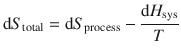
After multiplying with T on both sides of the equation, this yields:

or

The product −T ⋅ dS _total describes a new over-arching energy change for the underlying process and is called the Gibbs free energy change, which is defined as:

(2.42)

Since spontaneously occurring processes have a positive change in total entropy, the value of the Gibbs free energy change needs to be negative:

(2.43)

2.1.14 Inter-relatedness of Thermodynamic Quantities

From discussions in the previous sections we come to appreciate that the thermodynamic functions U, H, S, G and A of a given system vary with changes in the environmental functions T, p and V (assuming that the composition of the system remains constant). It also became clear that all thermodynamics properties are inter-related, and one can therefore describe any property as a function of two others.

A rigorous treatment of this issue reveals that there exist relationships between properties that are not apparently related. These relationships have been derived from basic equations of state by James Clerk Maxwell in 1870 and are thus termed the Maxwell relations. They are of tremendous practical importance when determining experimental values of quantities that are difficult to measure, such as entropy.