Physical Chemistry Essentials - Hofmann A. 2018

Interactions of Matter with Radiation
13.1 General Spectroscopic Principles

In Sect. 8.2.1, we already had a look at the interaction of atoms and electromagnetic radiation. Specifically, the atomic spectra were used to obtain insights into the inner fabric of atoms and their energetic states. Importantly, the spectral data provided the experimental verification of theoretical models such as the atomic model by Bohr (Sect. 8.2.2) and the quantum mechanics of the hydrogen atom by the Schrödinger equation (Sect. 10.1).

Since detailed information about structure, bonding and intra-/inter-molecular processes can be obtained from analysis of the interaction between matter and electromagnetic radiation, the area of spectroscopy is of fundamental importance for a wide variety of chemical disciplines.

13.1 General Spectroscopic Principles

In the study of matter and its interaction with electromagnetic radiation, two general processes can be distinguished:

✵ absorption describes the uptake of energy by an atom or molecule from incident electromagnetic radiation

✵ emission describes the release of electromagnetic radiation from an atom or molecule.

Either process is due to transitions between different energetic states; we have used this concept already in Sect. 8.2.2. The fundamental equation is therefore:

(13.1)

which means that in order to enable a transition from the lower (start) to the higher (end) energy level, electromagnetic radiation is required that possesses just the right quantum of energy ΔE. This is called the resonance condition.

When irradiating matter with light of appropriate energies, such transitions between discrete energy states occur as a consequence of either induced absorption or emission. Additionally, if a molecule has populated an excited state and it transitions back into the ground state, such transition might be accompanied by spontaneous emission of photons.

13.1.1 Intensity

A fundamental question of the interaction between radiation and matter addresses the loss of intensity of an incident beam as it travels through a sample of interest (Fig. 13.1). Practically, in most cases the sample will be contained in cuvette and potential interactions of the incident radiation with the cuvette material thus needs to be corrected for when conducting the experiment.

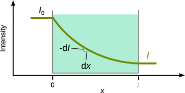
Fig. 13.1

Loss of intensity of an incident beam due to absorption

If the intensity of the beam at any point x on its way through the sample is I, the loss of intensity dI is proportional to the intensity at that point. Furthermore, dI is also proportional to the sample thickness dx penetrated:

Conversion of the proportionality to an equality relation requires the introduction of the proportionality constant μ (also known as the linear attenuation coefficient; see Sect. 13.6.2). Considering that the overall thickness of the sample shall be l and the intensity of the incident beam be I ₀, the above equation can be integrated between the boundaries of x = 0 and x = l after separating the integration variables I and x:

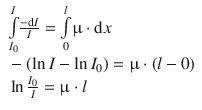
(13.2)

The natural logarithm of above equation is converted into a decadic logarithm, which yields:

(13.3)

known as the Bouger-Lambert law where a is the linear absorption coefficient. If the sample consists of a solution where the solvent shows no absorption of the incident radiation, the absorption coefficient depends on the molar concentration c of the radiation-absorbing solute:

and introduces the molar absorption coefficient ε, from which the law of Lambert-Beer is obtained:

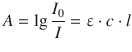
(13.4)

where A is called absorbance and the ratio of transmitted versus incident intensity is called transmittance: . The absorbance has no units and can in principle take infinite values; however, in experimental designs, only values of A < 2 deliver useful results, owing to the fact that the law of Lambert-Beer is only valid for comparably low concentrations (<0.5 M).

13.1.2 Intensity and Absorption Strength at the Molecular Level

A spectrum observed for a particular sample represents the superposition of a large number of transitions in individual atoms or molecules. The intensity of the observed absorption peaks therefore depends on the difference in the number of atoms/molecules occupying the two different energetic states. The ratio of these populations is given by the Boltzmann expression (see also Sect. 5.1.2)

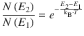
(13.5)

where N(E ₂) and N(E ₁) are the number of atoms or molecules in the excited (energy E ₂) and ground states (energy E ₁), respectively. The larger the difference in the population of the two states, the more intense the spectral peak will be.

From physics and radio communications it is known that in order to transmit or receive radio waves one requires an oscillating dipole and a dipole antenna, respectively. In addition, since radio waves emitted by an oscillating dipole are linearly polarised, the receiving dipole antenna needs to be oriented such that is in alignment with the plane of polarisation of the emitted signal. The emission and absorption of light (or generally electromagnetic radiation) by molecules follows the very same physical concepts. One can thus only expect absorption or emission of light by molecules that possess a dipole momentum. Typically, these will be permanent dipoles, but in some applications dipoles may also be induced in molecules that have no permanent dipole momentum. In cases involving linearly polarised light, one also needs to consider orientation effects.

Chromophores are the light absorbing moieties within a molecule. Due to differences in electronegativity between individual atoms, they possess a spatial distribution of electric charge. This results in a dipole momentum (ground state), such as for example the permanent dipole momentum of a carboxylic acid or an amide group (Fig. 13.2).

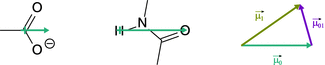
Fig. 13.2

Permanent dipole moment of the carboxyl group (left) and the amide bond (centre). Right: The permanent dipole momentum changes when the molecule transitions into an excited state. The difference vector between the permanent dipole momentum in the ground state () and the excited state () is called transition dipole momentum ()

When light is absorbed by the chromophore, the distribution of electric charge is altered and the dipole momentum changes accordingly (; excited state). The transition dipole momentum is the vector difference between the dipole momentum of the chromophore in the ground and the excited state. This transition dipole momentum is a measure for transition probability, and its dipole strength, D ₀₁, is defined is the squared length of the transition dipole momentum vector:

(13.6)

The strength of this transition dipole momentum is directly related to the probability with which a transition occurs, i.e. the strength of an absorption band. Spectroscopic data can thus be analysed to obtain numerical values for a transition dipole momentum which connects the absorption spectrum to the quantum mechanical wave function of a molecule.

13.1.3 Selection Rules

Owing to the underlying quantum mechanics, transitions between different energy states have to follow particular selection rules. Whereas allowed transitions possess a high probability of occurring, forbidden transitions are unlikely to occur. Forbidden transitions can be classified into spin-forbidden and symmetry-forbidden transitions.

Spin-forbidden Transitions

As we have seen earlier, the electronic states of atoms and molecules can be described by orbitals which contain up to two electrons paired with anti-parallel spin orientation. The total spin S is calculated as the sum of the individual electron spins (s _i ):

(13.7)

The spin multiplicity M is given by

(13.8)

and informs about the number of different possible arrangements of the unpaired spins in an external magnetic field (Table 13.1).

Table 13.1

Spin multiplicity of atoms and molecules

For a transition to be allowed, the spin multiplicity must not change, i.e.

(13.9)

Thus, a transition from a singlet to a triplet state and vice versa is normally forbidden.

Symmetry-forbidden Transitions

In Sect. 13.1.2 above, we have introduced the transition dipole momentum μ₀₁ the strength of which is a measure for transition probability. Quantum-mechanically, the transition dipole momentum is described as

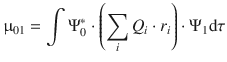
(13.10)

which tracks the positions (r _i ) of the electron charges (Q _i ) in the molecule. Ψ₁ is the wave function describing the molecular orbital of the excited state and Ψ*₀ is the complex conjugate wavefunction of the ground state; dτ = dx dy dz is the volume element. The wavefunctions inherently describe the symmetry of the molecular orbital. Unless the product 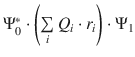is of a certain symmetry, the integral in Eq. 13.10 will be zero and therefore the strength of the transition dipole momentum will be zero, i.e. the transition will not occur. Transitions with D ₀₁ → 0 are called forbidden transitions, the probability of their occurrence is low. If D ₀₁ → 1, the transition is called allowed and occurs with high probability.

Symmetry rules and wavefunctions

When comparing the three wave functions in Fig. 13.3, it becomes obvious that Ψ₀ and Ψ₂ are symmetric with respect to their centre plane (mirror plane), but Ψ₁ possess no mirror symmetry (instead it possesses an inversion centre). The symmetry properties of wavefunctions are also known as parity.

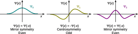
Fig. 13.3

The symmetry (parity) of wavefunctions

Ψ₀ and Ψ₂ are thus called ’symmetric’ or ’even’, and Ψ₁ is called ’anti-symmetric’ or ’odd’. In algebraic terms, this means:

✵ if f(x) = f(−x), then f is an even function;

✵ if f(x) = −f(−x), then f is an odd function.

When multiplying functions, the following rules apply:

✵ An even function times an even function yields an even function;

✵ an odd function times an odd function yields an even function;

✵ an even function times an odd function yields an odd function.

When dealing with wavefunctions, there are two general rules to be considered:

✵ The integral over all space for an even function is non-zero.

✵ The integral of an odd function over all space yields zero.

Using ethylene as an example, we can now use Eq. 13.10 to appraise a potential transition from the π to the π^* orbital of ethylene (Fig. 13.4):

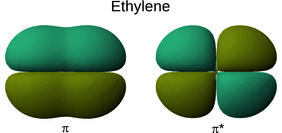
Fig. 13.4

The π and π^* orbitals of ethylene

Ψ^* ₀: The π orbital of ethylene is even.

Ψ₁: The π^* orbital of ethylene is odd.

(Q _i ·r _i ): The distribution of charge develops with distance and is therefore an odd function.

The product this yields: ’even’·’odd’·’odd’ = ’even’. The integral over the product is thus non-zero and the transition from the π to the π^* orbital in ethylene is allowed.

In contrast, if the molecular orbitals of the excited state had the same symmetry as those of the ground state, such as e.g. in butadiene, then transitions between those orbitals are forbidden based on the symmetry rules.

13.1.4 Line Width and Resolution

Theoretically, the two energy levels involved in a transition have discrete energy values which should result in a sharp spectral line. However, since the life time of the excited state of an atom or molecule is limited and much shorter than the life time in the ground state, the peak width broadens due to the Heisenberg uncertainty relationship (see also Sect. 8.1.6). Spectral lines thus have a non-zero width. Applied to transitions between energy levels, the uncertainty relationship is

(13.11)

where ΔE is and Δt are the uncertainties in determining the energy difference of a transition and life time of a particular state, respectively. The uncertainty relationship as given in Eq. 13.11 causes a natural line width Δλ₀ for a particular spectral transition. The uncertainty relationship enables us to calculate a minimum natural line width as per

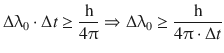
(13.12)

where Δt is the observation time.

In the recorded spectrum, the line shape follows a Lorentzian function. If the maximum intensity (=transition probability) for a transition is recorded at the central wavelength λ_c, then there will be a distribution of intensities given by the relationship

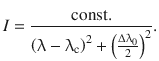
(13.13)

Additionally, the width of spectral lines may also be broadened by collisional processes or chemical reactions. For example, the absorption spectrum of a substance in its liquid state typically shows broader peaks than a spectrum obtained in the gas phase. Since the likelihood of collisions is larger in the liquid than in the gas phase, excited molecules are more readily deactivated and thus have a shorter life time.

As illustrated in Fig. 13.5, the peak width is typically defined as the width at half maximum (FWHM, full width at half maximum). From a practical perspective, it is important that two neighbouring peaks in a spectrum can be distinguished. This separation of two neighbouring peaks in a spectrum is called resolution. It is quantitatively measured by the resolving power, which in case of a wavelength-based spectrum is calculated as per:

(13.14)

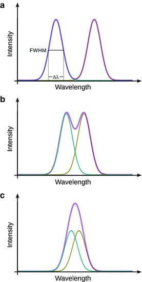
Fig. 13.5

Schematic explanation of full width at half maximum as well as the effect of resolution. (a) Two fully resolved peaks; (b) two overlapping peaks; (c) two non-resolved peaks. The red line indicates the observed spectrum which is the sum of the individual peaks

Here, Δλ is the difference between the wavelengths of the two neighbouring peaks λ₁ = λ and λ₂ = λ + Δλ.

13.1.5 The Electromagnetic Spectrum

Figure 13.6 shows the spectrum of electromagnetic radiation, organised in increasing energy from left to right. We have previously introduced the energy of a photon (Sect. 8.1.4) and can thus introduce the relationship between wavelength λ and wavenumber and the photon energy as per:

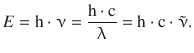
(13.15)

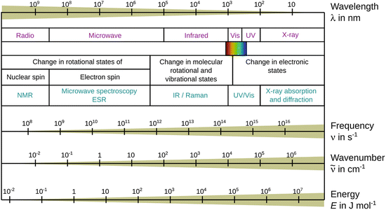
Fig. 13.6

The electromagnetic spectrum and the use of particular regions for spectroscopic applications

From this equation, we immediately appreciate that the frequency ν and the wavenumber increase with increasing energy, whereas the wavelength gets shorter the higher the energy of the radiation.

Different types of interactions happen between electromagnetic radiation of certain energy regions with matter. The various interactions with matter and the appropriate types of spectroscopy are mapped to the electromagnetic spectrum in Fig. 13.6.