Physical Chemistry Essentials - Hofmann A. 2018
Interactions of Matter with Radiation
13.3 Rota-vibrational Spectroscopy
13.3.1 The Rotational Spectrum
In Sect. 9.2.2 we discussed the rigid rotor with space-free axis which we now consider as a model to describe the rotation of a two-atomic molecule. This model assumes that the two atoms are bonded to each other at a fixed distance (’rigid’) and that the axis of the two-atomic molecule is allowed to take any orientation in an outside coordinate system (’space-free axis’) while the centre of gravity rotates around the origin. Equation 9.29 delivered the allowed energy levels of such a rotor as
![]()
(9.29)
whereby the rotational constant
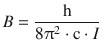
(13.24)
is dependent on the momentum of inertia I; h and c are the Planck constant and the speed of light, respectively. In order for a transition between different rotational levels to occur, the resonance condition needs to be met; i.e. electromagnetic radiation of the matching energy needs to be provided to (absorption spectrum) or is released from (emission spectrum) the molecule. Second, we need to consider relevant selection rules as there are many different rotational levels between which transitions could potentially occur.
The selection rules define that only transitions with ΔJ = ±1 are possible. If we assume a starting level of J start and an end level of J end = J start + 1, we can calculate the resonance energy for a transition:
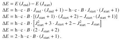
(13.25)
Using the relationship in Eq. 13.15, we can thus calculate the wavenumber of a transition between the two rotational levels J and (J+1) as per:
![]()
(13.26)
This equation allows a conclusion as to the appearance of a rotational spectrum. For the transition of rotational level 0 to level (0 → 1) we are expecting a peak in a plot of absorbance versus wavenumber that is spaced at a distance of 2·B from ![]() = 0. For transition 1 → 2 the peak is spaced 4·B from
= 0. For transition 1 → 2 the peak is spaced 4·B from ![]() = 0, etc. In other words, Eq. 13.26 predicts a spectrum with peaks with a distance of 2·B between them (see Fig. 13.14). In reality, the distance between the absorption peaks decreases as the wavenumber increases, owing to the fact that the molecule is indeed not a rigid rotor as assumed in the above model. At higher rotational states, the distance between the two atoms (and thus the momentum of inertia I = m · r 2, Eq. 9.7) increases due to the centrifugal force. As per Eq. 13.24 above, an increase in I prompts a decrease in B (see analysis of rota-vibrational spectra in Sect. 13.3.4).
= 0, etc. In other words, Eq. 13.26 predicts a spectrum with peaks with a distance of 2·B between them (see Fig. 13.14). In reality, the distance between the absorption peaks decreases as the wavenumber increases, owing to the fact that the molecule is indeed not a rigid rotor as assumed in the above model. At higher rotational states, the distance between the two atoms (and thus the momentum of inertia I = m · r 2, Eq. 9.7) increases due to the centrifugal force. As per Eq. 13.24 above, an increase in I prompts a decrease in B (see analysis of rota-vibrational spectra in Sect. 13.3.4).
To appreciate the type of electromagnetic radiation that fulfils the resonance condition for a rotational spectrum, we consider the molecule HCl which possesses a bond length of 1.29 Å. This yields a momentum of inertia of

The rotational constant of HCl is then
For the transition from the rotational ground to the first excited state (0 → 1), the following wavenumber can be computed by using Eq. 13.26:
![]()
and converted into a wavelength or frequency
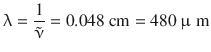
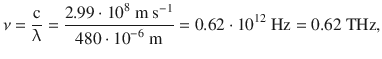
corresponding to a resonance energy of ΔE = 4.1·10−22 J. These values indicate that rotational transitions in molecules require a resonance energy in the range of microwaves and far infrared. Purely rotational spectroscopy is thus often called microwave spectroscopy (Fig. 13.13).
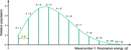
Fig. 13.13
Wavenumbers for transitions in a rotational spectrum (see Eq. 13.26). The absorption of individual transitions is based on the relative absorption of the starting states as given in Eq. 13.27
If the transition moment is the same for all different starting levels J (which is indeed the case), then the intensity of individual peaks in the rotational spectrum should be dependent on the population of the starting level of the transition that elicits an individual peak. However, one needs to remember that the quantum mechanical discussion of the rigid rotor resulted in several degenerate states, whereby (2J + 1) states of the same energy were possible for each state J (see Sect. 9.2.2). This degeneracy has to be accounted for in addition to the Boltzmann expression that describes the ratio of population of a rotational state J with respect to all states:
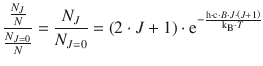
Using the above equation, the population ratio of N J /N and N J=0/N can be evaluated, and the quotient of both ratios yields the ratio of populations of state J and state J = 0:
(13.27)
For HCl at T = 293 K with B = 10.4 cm−1 the relative population of state J = 1 with respect to J = 0 is then:
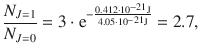
which means that the population of the rotational level J = 1 is 2.7 times higher than the rotational ground state J = 0. The peak intensity in the rotational spectrum thus progresses through a maximum value with increasing J, as indicated in Fig. 13.14.
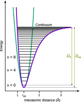
Fig. 13.14
Comparison of the potential energy of the harmonic (blue) and anharmonic (red) oscillator
13.3.2 The Vibrational Spectrum
The quantum mechanical background for vibrational modes of molecules are given by the harmonic oscillator which we discussed in Sect. 9.3 where we derived the discrete energy levels in dependence of the vibrational quantum number v as
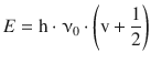
(9.38)
whereby the oscillation frequency ν0 is a function of the force constant k and the reduced mass μ:
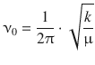
(9.34)
The selection rule for vibrational transitions is Δv = ±1, allowing only transitions between neighbouring vibrational levels. The resonance energy required for a transition from vstart to vend = vstart + 1 is thus:
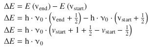
(13.28)
The frequency of the electromagnetic radiation fulfilling the resonance condition is thus the same as the frequency of the vibrational mode of the molecule. Using again HCl (k = 480.6 N m−1) as an example, the type of energy required for vibrational resonance can be calculated:
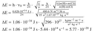
This corresponds to a wavelength and wavenumber of:

thus indicating that the resonance energies are in the region of the infrared.
The resonance energy for a vibrational transition is thus two orders of magnitudes higher than that required for transition between two rotational states. This has substantial implications for the relative population of the individual vibrational states. In analogy to the discussion of the electron/nuclear magnetic states (Table 13.4) as well as the rotational states (Eq. 13.27), this can be calculated using the Boltzmann statistics:
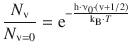
(13.29)
For HCl at T = 293 K with ν0 = 0.87·1014 Hz, the relative population of state v = 1 with respect to v = 0 is then:
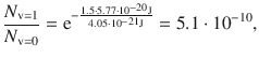
indicating that at room temperature virtually all molecules occupy the vibrational ground state.
13.3.3 Anharmonicity
A closer look at Eq. 13.29 shows that at increasing temperatures one expects that the population of vibrationally excited molecules will be continuously increasing. It should thus be possible to store ever higher energy in molecules which would undergo ever more intense vibrations. This situation is in contradiction to experimental observations: we know that molecules dissociate (i.e. the distance between atoms becomes very large) if they are exposed to high enough temperature.
We remember that the model we used to describe vibrational modes of a di-atomic molecule is based on the harmonic oscillator (see Eq. 9.33 and Fig. 9.9). Graphically, this is illustrated by a symmetric potential curve where the potential energy develops with the square of the distance between two bonded atoms:
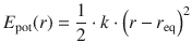
(13.30)
where the equilibrium bonding distance between the two atoms is r eq, and k is the force constant.
Two adjustments of the harmonic potential are required to describe the real behaviour of molecular vibration (see Fig. 13.14):
✵ Even at high energy levels, the distance between the two atoms cannot get arbitrarily small. The Coulomb repulsion between the two nuclei prevents very small inter-atomic distances. The left branch of the parabolic function thus needs to develop steeper than suggested by the harmonic potential.
✵ The right branch of the potential function needs to progress into a horizontal line at an energy level that represents the dissociation energy. When the molecule reaches this vibrational state, the distance between the two atoms can become arbitrarily large.
The resulting function describes a so-called anharmonic oscillator. At low energy levels, an anharmonic oscillator behaves very similar to a harmonic oscillator. At higher energies, substantial deviations from harmonicity are observed. The energy difference between the minimum of the potential energy curve and the horizontal branch equals the dissociation energy D eq. Since any bond possesses a zero point energy
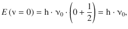
the first vibrational level is elevated by h·ν0 from the minimum of the potential energy curve. The experimentally relevant dissociation energy is thus D 0 which is the difference between the vibrational ground state and the horizontal branch of the potential curve.
The potential curve of the anharmonic oscillator cannot be rigorously derived. The Lennard-Jones potential (see Sect. 11.5 and Fig. 11.8) is one model to describe the potential energy function of an anharmonic oscillator. Another very frequently used function is the Morse function
![]()
(13.31)
which features the dissociation energy D eq and the constant β as a modified force constant (see also Eq. 9.37). Mathematically, the above function can be developed into a so-called Maclaurin series:

which shows high similarity with the potential energy function for the harmonic oscillator above (Eq. 13.30); the anharmonicity correction results from additional terms with (r−r eq )3, (r−r eq )4, etc. Using this Morse potential to solve the Schrödinger equation, the following energy eigenvalues are obtained for the anharmonic oscillator:
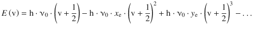
(13.32)
with the anharmonicity constants x e and y e.
The anharmonicity has two major implications:
✵ The selection rules are different from those of the harmonic oscillator, owing to a different wavefunction. The selection rules for the anharmonic oscillator allow further transitions with Δv = ±1, ±2, ±3, …
✵ A transition with Δv = ±1 is called fundamental; transitions with Δv = ±2, ±3, … are called overtones.
✵ Due to the presence of additional terms with power 2 and higher in Eq. 13.32, the distance between consecutive vibrational levels is not constant but decreases with increasing quantum number v. Therefore, there is only a finite number of vibrational levels until the dissociation energy is reached.
13.3.4 The Rota-vibrational Spectrum: Infrared Spectroscopy
The discussion of the pure rotational and pure vibrational spectra in the previous sections showed that the resonance energy required for vibrational excitation is by about two orders of magnitudes larger than that required for rotational excitation. One can thus expect that upon vibrational excitation vibrational modes will also be excited. The observed vibrational spectra therefore consist of peaks rather than lines. If sufficient spectral resolution can be achieved, the vibrational peaks show a structure that can be analysed as to rotational transitions. The resulting spectra are thus called rota-vibrational spectra.
In infrared spectroscopy, the probing of rota-vibrational transitions is carried in an absorption experiment where samples are exposed to infrared light and the absorbance is monitored. Since vibrational as well as rotational transitions will be observed, one needs to consider the selection rules for the vibrational quantum number as well as those for the rotational quantum number; for the purpose of the following discussion, we are ignoring the possible overtones due to anharmonicity:
✵ Δv = ±1
✵ ΔJ = ±1.
Figure 13.15 shows two vibrational states v = 0 and v = 1 and overlayed on each the rotational states. It is obvious that when transitioning from vstart = 0 to vend = 1, there are two ways to satisfy the rotational selection rule; one can start from a lower rotational state and transition to the next higher rotational state (J start = 0, J end = 1) or vice versa (J start = 1, J end = 0). This gives rise to two different blocks of transitions (called branches) which are grouped at lower ( P-branch) and higher ( R-branch) energies, respectively.
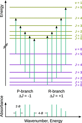
Fig. 13.15
Top: Rotational transitions for the excitation of the first vibrational state from the vibrational ground state. Bottom: The resulting schematic rota-vibrational spectrum
The wavenumbers for the two different branches can be calculated considering Eqs. 13.25 and 13.28:
In exceptional cases, e.g. when molecules exist in triplet state (where the total electron spin is not zero), the selection rules may also include Δv = ±1 and ΔJ = 0. In such cases, a third branch called Q-branch is observed.
A close look at the expressions in Table 13.6 shows that a wavenumber ![]() that corresponds to the pure vibrational transition (
that corresponds to the pure vibrational transition (![]() ) is not possible, i.e. the pure vibrational transition is not observed, since ΔJ = 0 is not allowed in the absence of a Q-branch. This gives rise to the so-called zero gap of the rota-vibrational spectrum; the distance between the two first peaks of the P- and R-branches is:
) is not possible, i.e. the pure vibrational transition is not observed, since ΔJ = 0 is not allowed in the absence of a Q-branch. This gives rise to the so-called zero gap of the rota-vibrational spectrum; the distance between the two first peaks of the P- and R-branches is:
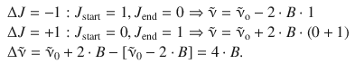
Table 13.6
Wavenumbers for rota-vibrational transitions
|
P-branch |
R-branch |
Δv = +1, ΔJ = −1 |
Δv = +1, ΔJ = +1 |
|
|
Figure 13.16 depicts the rota-vibrational spectrum of HCl and shows two particular details. First, there are two peaks for each individual vibrational transition, owing to the fact that HCl is a mixture of two isotopes H35Cl and H37Cl. H37Cl has a slightly larger reduced mass than H35Cl (but the same force constant). According to Eqs. 13.24 and 13.26, this results in a lower frequency and hence a smaller wavenumber.
Fig. 13.16
Rota-vibrational infrared spectrum of HCl. The peaks of individual transitions are split into two with the less intense peaks (at lower energies) belonging to isotope H37Cl and the more intense peaks (at higher energies) arise from H35Cl
Second, the distance between the vibrational peak clusters decreases with increasing wavenumber; this cannot be explained by an effect of higher vibrational levels as in that case, the effect should be symmetric in the P- and R-branch with respect to the zero gap. The explanation for this effect becomes obvious when comparing the harmonic and anharmonic oscillator potential curves (Fig. 13.14). The potential curve for the anharmonic oscillator is symmetric with respect to the equilibrium distance r eq; when moving to higher vibrational levels, the equilibrium distance remains constant. In case of the anharmonic oscillator this is different. Excitation of higher level vibrational modes leads to an increase in the bonding distance. With an increase in distance between the two bonded atoms, there is an increase in the momentum of inertia and thus a decrease of the rotational constant B (Eq. 13.24). The rotational constant is therefore dependent on the vibrational mode and its decrease with larger quantum numbers v is reflected in a decrease of the distance between peaks in the rota-vibrational spectrum.
We thus conclude that in order to explain all observations in the rota-vibrational spectrum, we not only need to replace the harmonic with the anharmonic oscillator model, but also the rigid rotor with the non-rigid rotor model.
13.3.5 The Rota-vibrational Spectrum: Raman Spectroscopy
In the discussion of general concepts of absorption spectroscopy in Sect. 13.1.2, we mentioned that an interaction of incident electromagnetic radiation with a molecule (= absorption) only happens if the molecule possesses a dipole momentum. This means that
✵ homonuclear two-atomic molecules (e.g. O2, Cl2, etc)
✵ symmetric multinuclear linear molecules (e.g. CO2)
✵ fully symmetric multinuclear molecules (e.g. CH4)
possess no rotational absorption spectrum due to the absence of a dipole momentum. Furthermore, homonuclear two-atomic molecules possess no vibrational absorption spectrum either.
However, in this discussion it was implied that the light-absorbing matter needed to possess a permanent dipole momentum which changes upon interaction with incident electromagnetic radiation, thus giving rise to a transition dipole momentum and hence absorption.
We now consider the possibility that the interaction of incident radiation can induce a dipole momentum in a molecule. This phenomenon results in a similar situation, namely that there has been a change in the dipole momentum. The induced dipole momentum μind can be calculated as per
![]()
(11.18)
where E is the electrical field strength and α is the polarisability, a quantity we have discussed earlier (see Sect. 12.2.1).
If the electrical field E at the molecule arises due to an electromagnetic wave (with energy h·ν), the field changes periodically with the frequency ν and so does the induced dipole momentum μind. In turn, the dipole momentum μind oscillating with frequency ν causes emission of light with the energy h·ν. Therefore, the molecule emits light of the same energy that it is being exposed to. This effect is known as Rayleigh scattering and macroscopically appears as an elastic scattering of light by an object.
However, if an energy transfer between incident radiation and molecule happens during this process, the resulting scattering is inelastic, i.e. the energy of the emitted light has different energy than the incident light; this is called the Raman effect. It had been predicted by Adolf Smekal (Smekal 1923) and experimentally proven by Sir Chandrasekhara Venkata Raman. Two situations can arise:
✵ The incident photon transfers energy onto the molecule which, in turn, transitions into a higher energy state. The emitted light thus has lesser energy than the incident light. This gives rise to the so-called Stokes lines (or S-branch).
✵ The incident photon gains energy from the molecule which transitions from a state of higher energy to a state of lower energy. The emitted light here has higher energy than the incident light, giving rise to the anti-Stokes lines (or O-branch).
The energy levels between which such transitions occur are the rotational levels as well as the vibrational levels. Therefore, the energy difference between incident and emitted light corresponds to the energy difference between the rotational (and vibrational) levels between which the transition occurs.
The selection rules for rota-vibrational transitions in the Raman effect are
✵ Δv = ±1
✵ ΔJ = 0, ±2
Since it is the energy difference between the incident light and the emitted light that contains the information about the rota-vibrational transitions in the molecule, Raman spectra are interpreted based on the ΔE (or Δν). This is called the Raman shift and obtained as difference between an individual peak and the energy or wavenumber of the incident light which features as the Rayleigh scattering peak in the Raman spectrum.
For a rotational transition J start → J end with J end = J start + 2, the wavenumber can be quantum mechanically calculated based on the rotational quantum number as per
(13.33)
For J start = 0, this yields for the first Stokes line:
and for the first anti-Stokes line:
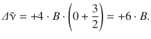
It is thus obvious, that the rotational Raman spectrum (Fig. 13.17) features the first Stokes and anti-Stokes lines in a distance of 6·B from the Rayleigh scattering peak. The peaks for the following transitions are then spaced at a distance of 4·B from each other.

Fig. 13.17
Simulated rotational Raman spectrum of N2. If light with a wavenumber of 2358 cm−1 is used as incident beam, the spectrum would feature a broad Rayleigh scattering peak at this wavenumber. The N-N triple bond vibration occurs at 2358 cm−1
The angular dependency of the Raman scattering intensity is given by the relationship
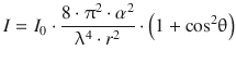
(13.34)
where I 0 is the intensity of the incident beam at wavelength λ, α is the polarisability, r the distance of the sample to the detector and θ the angle between the incident and the scattered ray. The function cos2θ oscillates between the values of 0 and 1 and assumes 0 at 90°, and the function (1 + cos2θ) thus has its lowest values at 90° and 270° (see Fig. 13.18). Therefore, the scattering intensity at right angles is half the scattering intensity in forward direction.
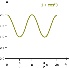
Fig. 13.18
The function (1 + cos2θ) oscillates between values of 1 and 2
13.3.6 Conclusion
Infrared and microwave spectroscopy on the one hand and Raman spectroscopy on the other are useful tools that allow determination of force constants and atomic distances in bonds. The former methods require a change in the permanent dipole momentum of a substance during transition between different rotational or vibrational states. In contrast, Raman spectroscopy requires a change of the polarisability during the transition. Therefore, the two types of rota-vibrational spectroscopic methods are often complementary.
The vibrational spectra of molecules are typically rather complex and therefore assure that two different molecules have different vibrational spectra. Among other applications, this can be used very effectively in technique called fingerprinting. The vibrational spectrum of an unknown substance is acquired using either infrared or Raman spectroscopy and then compared with a database of reference spectra. If a match is found, the unknown substance can be identified.