Physical Chemistry Essentials - Hofmann A. 2018

Interactions of Matter with Radiation
13.6 Atomic Spectroscopy

The interactions of matter with radiation discussed in this chapter so far mainly focussed on molecules; the resulting spectroscopic methods are therefore invaluable for the investigation of structure and properties of molecular matter. However, there also particular interactions between electromagnetic radiation and single atoms. These interactions and the spectroscopic methods arising will be the subject of this section, and also close the loop to some observations and concepts we have discussed earlier. At few previous instances we have made reference to atomic spectra. In Sect. 8.2.1, we used atomic spectroscopy to learn about the fabric of atoms, and in Sect. 10.3.2, we discussed the ionisation energies of elements (derived from atomic spectroscopy) and the concept of shells. Furthermore, the importance of atomic spectroscopy for the study of surfaces and surface processes was in Sect. 7.3.

Clearly, there will be two types of electrons that can reveal information about the particular atoms studied. If the radiation used is of relatively low energy (such as in the optical spectra), the electrons investigated will be those of the outer ( valence) shell, i.e. those that define the chemical behaviour of an atom. Radiation of high energy, in contrast, will be probing the tightly bound electrons in the inner ( core) shells.

13.6.1 Optical Spectroscopy

When we considered the line spectrum of hydrogen in Sect. 8.2.1, we learned that the different spectral series observed with hydrogen in either atomic absorption or emission spectroscopy followed a particular relationship

(8.14)

whereby R_∞ is the Rydberg constant, and n ₀ and n are the principal quantum numbers of the lower and higher energy states, respectively, between which an electronic transition occurs.

If we now consider heavier atoms that also possess only one electron like hydrogen, such as

we appreciate that their fabric is very similar to that of hydrogen. The difference is that these ions possess a heavier nucleus and multiple nuclear charges (order number Z > 1). Their spectra can be observed under extreme conditions, for example when studying the light of stars. The spectra of these one-electron atoms are very similar to that of hydrogen, but the individual lines are shifted to higher frequencies. Importantly, the values of the Rydberg constant for those heavier ions differs from that of hydrogen. The reason for this discrepancy is that when deriving R_∞ it is assumed that an electron of mass m_e orbits around a nucleus of indefinitely high mass; therefore, the nucleus is assumed non-moving. However, nuclei with a real mass m _nucleus rotate together with the orbiting electron around the centre of gravity. Instead of the mass of an orbiting electron (m_e), one needs to use the reduced mass (see Sect. 9.2.1), which in this case is given as

The Rydberg constant for atoms with real mass m _nucleus is therefore obtained as

(13.44)

For optical transitions in heavier atoms (than hydrogen) with one electron, one also needs to consider that the nuclear charge is greater than +1e. The field experienced by the orbiting electron is thus different than in the case of hydrogen and depends on the nuclear charge, represented by the order number Z. Equation 8.13 therefore needs to be adjusted for the heavier one-electron atoms and then becomes

(13.45)

The spectra of atoms with more than one electron are more complicated than those of atoms with just one electron. The wavelengths at which individual lines appear in atomic emission or absorption spectroscopy are, of course, again given by the difference between the energies of the two states between which the transition occurs. However, compared to the fairly simple spectrum of hydrogen-like atoms (see above), the number of lines observed with multi-electron atoms is much larger and can be explained by superposition of different series. Historically, the individual terms (i.e. energy levels) have been called S ( sharp), P ( principal), D ( diffuse) and F ( fundamental); the explanation of these different series in terms of the principal quantum number n is illustrated in Table 13.8 (see also Fig. 13.26).

Table 13.8

Term series in optical spectroscopy, illustrated using sodium as an example

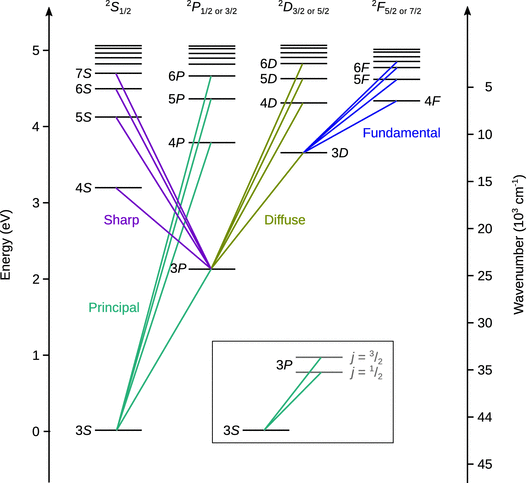
Fig. 13.26

The term scheme of sodium. The inset shows the dublet splitting of lines in spectra of alkali metals due to spin-orbit coupling

Optical Spectra of Alkali Metals

The optical spectra of alkali metals are quite similar to that of the hydrogen atom, owing to the fact that only one electron is responsible for the electronic transitions giving rise to these spectra. In this context, the nucleus and the non-valence electrons are often seen as an entity called the atomic core. The core electrons shield the nuclear charge up to the effective nuclear charge (1 e in case of the alkali metals). The effective nuclear charge is compensated by the valence electron. However, in contrast to the hydrogen atom, the effective nuclear charge experienced by the valence electron is not a point charge. The potential depends on the relative location of the valence electron with respect to the core and is therefore no longer of spherical symmetry. As a consequence, the n ² different energy levels (see Eq. 10.8) are no longer degenerate, and assume different values depending on the orbital angular momentum l.

Therefore, the spectroscopic terms S, P, D and F are linked to orbital quantum number l, in a similar fashion like the atomic orbitals (see Table 10.5). In order to avoid confusion, atomic orbitals are denoted in lower case and spectroscopic terms in upper case letters (Table 13.9):

Table 13.9

The spectroscopic terms and the orbital quantum number. Possible values of the quantum number for the total angular momentum for atoms with one valence electron are also given

In Sect. 10.2.3, we discussed the phenomenon of a magnetic field arising from the motion of a charged particle (electron) that spins around its own axis. This magnetic field couples with the magnetic field arising from the orbiting motion of the electron around the atomic nucleus. This spin-orbit coupling led us to introduce the total angular momentum , characterised by the quantum number j that can assume the values

(10.22)

Obviously, we need to consider this phenomenon when assessing the possible transitions of a valence electron. The selection rules for the optical spectra of the alkali metals are thus:

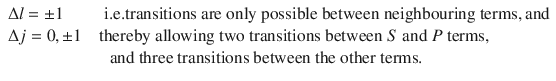
(13.46)

The different possible transitions are illustrated in the term scheme of sodium (Fig. 13.26). In spectroscopy, the individual quantum states are denoted with symbols such as

In this nomenclature, the spin multiplicity M = 2 · Σ s _i + 1 (Eq. 13.8) is shown as superscript. Then, the spectroscopic term (dependent on the orbital quantum number l) is given and the quantum number of the total angular momentum (j) is appended as subscript. Since alkali metals have just one valence electron, the total spin is thus Σ s _i = ½ and the spin multiplicity is M = 2; such terms are called dublet terms.

Optical Spectra of Multi-electron Atoms

In the context of optical spectroscopy, multi-electron atoms are those that possess more than one valence electron. The optical spectra of such atoms are thus much more complicated than those of single-electron atoms, since there are multiple term systems.

In the case of lighter atoms, the orbital momenti of individual electrons couple to form a total orbital momentum . Similarly, the spin momenti of individual electrons couple to yield a total spin momentum . Both of those total momenti then form a total angular momentum . This coupling is called Russel-Saunders coupling or L-S-coupling.

Heavier atoms possess a larger nuclear charge and therefore the spin-orbit become as strong as the interactions between individual spins or orbital angular momenti. In such cases, the orbital momenti and spin momenti of individual electrons tend to couple to form individual total angular momenti . These individual total momenti j then form a total angular momentum , hence this phenomenon is called j—j-coupling.

The selection rule for allowed transitions in multi-electron atoms is

(13.47)

13.6.2 X-ray Spectroscopy

The energy required to elicit emission of optical spectra from atoms may be provided in the form of thermal energy such as in the flame of a Bunsen burner, a plasma or by a discharge lamp. As discussed in the previous section, the energy difference in the quantum states of valence electrons as of the same order as that of the thermal energy and therefore the spectra arising from transitions of the valence electrons appear in the range of optical and UV light.

If atoms are exposed to electron beams of much higher energy (10 keV—100 keV), emission of light at much shorter wavelengths ( X-rays) is observed. Notably, this emission of X-ray light consists of two components, light that contains a continuous distribution of wavelengths (also known as Bremsstrahlung) as well as characteristic X-ray emission at particular wavelengths (see Fig. 13.27).

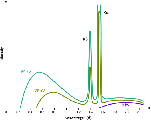
Fig. 13.27

X-ray spectrum obtained with a copper anode and electron beams of increasing energy. The shortest observed wavelength of the continuous X-ray spectrum shifts to higher energies as the kinetic energy of the incoming electrons is increased. At the same time, the intensity at individual wavelengths increases. Note that the wavelengths of characteristic X-ray emission remain constant

When accelerated electrons impact on matter they are slowed down by the electric fields of individual atoms. This deceleration results in a loss of kinetic energy which is released in the form of photons. The different wavelengths of the released photons thus result from the different kinetic energies of impacting electrons. Therefore, a minimum wavelength is observed in the Bremsstrahlung; this wavelength corresponds to the highest kinetic energy in the energy distribution of the impacting electrons.

A second process arising from the impact of high energy electrons onto matter is the displacement of an electron from the atomic core (i.e. from an inner shell). The vacated position is subsequently filled by an electron from an outer shell. This transition between two energy levels is accompanied by emission of a photon whose energy equals the energy difference between the two levels of this transition. The light emitted due to this latter process constitutes the characteristic X-ray emission of an element.

The individual lines of the characteristic X-ray emission can be classified into different series that depend on the principal quantum numbers (shells) of the two energy levels involved in the transition of the electron that fills the gap arising from the impact of high energy electrons (see Fig. 13.28). As with the optical spectra, the orbital angular momentum (represented by the quantum number l) and the total angular momentum (represented by the quantum number j) give rise to a fine structure, hence the selection rules for possible transitions are the same as for the optical spectra:

(13.46)

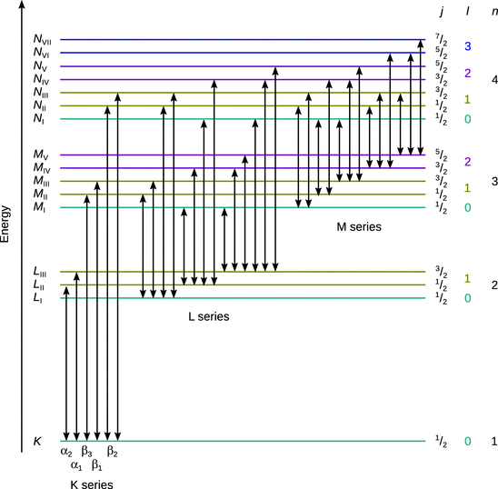
Fig. 13.28

Illustration of the allowed electron transitions resulting in the X-ray spectrum of atoms

The emission of characteristic X-ray photons can also be elicited by directing X-ray light onto matter. In this case, the process of X-ray emission is called X-ray fluorescence.

The naming of the lines in X-ray spectra frequently uses the traditional Siegbahn notation which denotes the shell of the high energy level as an upper case character (e.g. K) and appends Greek letters (α, β, …) as well as numerical indices. Since this notation is non-systematic, it often appears confusing. A more systematic nomenclature has thus been recommended by IUPAC (see Table 13.10).

Table 13.10

Naming of characteristic lines in X-ray spectra

The Mass Attenuation Coefficient

In Sect. 13.1.1 we saw that there is a loss of intensity as light travels through a sample of interest. The intensity of the exiting beam can be calculated from Eq. 13.2 and is given as per

(13.48)

where l is the thickness of the material (in cm) and μ the ( linear) attenuation coefficient (in cm⁻¹) which comprises of two components: the absorption coefficient τ and the loss off intensity based on scattering (σ). For X-rays, the scattering attenuation is negligible, therefore μ ≈ τ.

Since the attenuation is dependent on the mass of matter that is penetrated by the incident beam, the attenuation coefficient is often normalised with respect to the density ρ, thus yielding the so-called mass attenuation coefficient:

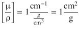
(13.49)

The mass attenuation coefficient is characteristic for a particular element and independent of the chemical and physical state of the sample. In mixtures and compounds, the mass attenuation coefficient is an additive property and therefore be calculated based on the molar ratio of the individual elements in the sample.

Notably, the mass attenuation coefficient depends on the wavelength of the incident radiation (Fig. 13.29). Moving from longer to shorter wavelengths (i.e. from lower to higher energy), the value of the mass attenuation coefficient continuously decreases, until the energy of the incident radiation is sufficient to remove an electron from the next inner shell; at this point, a strong increase in the mass attenuation coefficient is observed, giving rise to a so-called absorption edge. Further increase in the energy of the incident light leads to a renewed decrease of the mass attenuation coefficient until the energy is sufficient for displacement of an electron from the next inner shell.

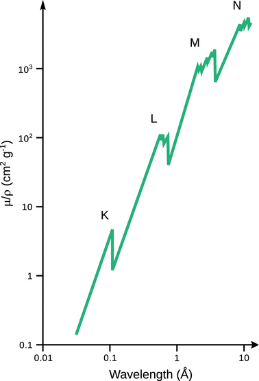
Fig. 13.29

The X-ray absorption spectrum of molybdenum

Moseley’s Law

The concepts discussed in the above sections have been concerned with X-ray spectra observed with a particular atom. An important discovery was made by the British physicist H enry Moseley in 1913, when he compared the energies of particular lines, e.g. the Kα₂ transition, of different elements (Moseley 1913). Expressing the energies of these transitions as either the frequency or wavenumber, a linear correlation between the square root of either ν or with the order number Z is found:

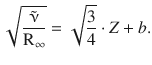
(13.50)

For a particular transition between two shells with the principal quantum numbers n _high (the inner shell) and n _low (the outer shell), the law can be formulated as:

(13.51)

Interestingly, the term (Z-a) suggests that there is a correction with respect to the positive charge (given by the number of protons = order number). This correction makes sense when we consider that an electron jumping from the outer to the inner shell experiences only the effective nuclear charge, since electrons in inner shells shield the nuclear charge to some degree. This shielding effect is captured by the constant a.

For example, for the Kα transition (principal quantum numbers n _high = 1 and n _low = 2), an electron jumps from the L- to the K-shell to fill a gap caused by a displaced electron. There is one remaining electron in the K-shell and provides a shielding of the nuclear charge by about 1·e. Consequently, the constant a is found to be approximately 1 for this transition.

13.6.3 Auger Electron Spectroscopy

In Sect. 7.3.2, we have introduced the technique of Auger electron spectroscopy as a method to investigate surface processes. The Auger phenomenon arises as an alternative pathway when core electrons are displaced by impact of high energy electrons or photons. As discussed above, the displacement of an inner shell electron leads to the transition of an electron from an outer shell to fill the gap closer to the nucleus. The energy released during this transition can be emitted in form of a photon (characteristic X-ray lines), but also be transferred onto another electron which is then departing from the atom due to its high energy. Although this process was discovered independently by Lise Meitner (Meitner 1922) and Pierre Auger in the 1920s, it has historically been credited to Auger; the emitted electron is thus called the Auger electron. Auger electron emission and X-ray photon emission are two competing processes. The Auger electron emission typically dominates in lighter atoms, whereas X-ray emission is the preferred process in heavier atoms.

As a consequence of the outlined Auger process, the kinetic energy of the emitted electron equals the energy difference between the two levels involved in the transition of the electron that closes the gap in the inner shell. Notably, this energy is not identical with the energy of a characteristic X-ray photon in the X-ray process. Whereas the latter results in an atom with one positive charge (due to the electron displaced by the impacting high energy electrons), the Auger process results in a doubly charged ion (due to one displaced electron and one emitted Auger electron).

In order to characterise individual Auger process, three electron states need to be described:

✵ the first state denotes the state from which the primary electron is dislodged

✵ the second state describes where the electron originates from that fills the inner shell gap

✵ the third state identifies the level from which the Auger electron originates.

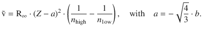
For example, the the Auger spectrum of palladium shows three distinct peaks (Fig. 13.30). For all three types of Auger electrons, a hole is generated in the K-shell by impact of high energy electrons. This core hole can be filled by transition of an electron from either the L _I , L _II or L _III levels. The energy released during that transition is then transferred to an electron in one of the L levels which is then emitted as an Auger electron from the atom.

Fig. 13.30

(a) Schematics of particular Auger processes. (b) Auger spectrum of palladium based on data by Babenkov1982. The inset shows the differentiated form of the Auger spectrum

The kinetic energy of Auger electrons is measured by electron energy analysers which are typically based on retardation or deflection of the emitted electrons as they pass through a variable electric or magnetic field. The degree of retardation or deflection is proportional to the kinetic energy. Electrons detected at a particular energy are then directed into an electron multiplier for analysis. Frequently, Auger spectra are measured in a differentiated form (Fig. 13.30b, inset) which allows for a more sensitive detection of peaks.

Importantly, the emission of Auger electrons is not dipole radiation and, therefore, selection rules such as those observed with X-ray emission do not apply. The energy of a particular Auger electron is given by

(13.52)

where E _hole is the energy of the electron being displaced, E _second is the energy of the electron replacing the dislodged electron and E′_binding is the binding energy of the Auger electron in the atom, corrected for the doubly charged state of the atom. Note that the energy of the impacting electron is not featured in Eq. 13.52, since it does not affect the energy of the emitted Auger electrons. The only requirement is that the energy of the impacting electron is sufficiently large to displace an electron from a core shell. The energy of the impacting electron thus needs to be at least as high as the binding energy of the electron to be displaced.

Equation 13.52 shows further that the energies of Auger electrons arise as characteristic for particular elements. Auger electron spectra are thus valuable tools for identification of atoms (see also Sect. 7.3.2), but also for measuring energy levels of the different shells.