Physical Chemistry Essentials - Hofmann A. 2018
Appendix A Mathematical Appendix
A.1 Basic Algebra and Operations
A.1.1 Exponentials
Definitions
a n = a · a · a · a … · a |
|
a 1 = a |
|
a 0 = 1 |
|
a − n = 1/ a n |
Computation rules
a x a z = a x + z |
a x b x = ( ab ) x |
|
|
( a x ) z = a x ⋅ z |
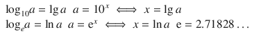
A.1.2 Logarithm
Definition
![]()
Special cases
Computation rules
log b ( u ⋅ v ) = log b u + log b v |
|
log b ( u z ) = z ⋅ log b u |
|
Change of base
![]()
A.1.3 Nonlinear Equations
The quadratic equation a ⋅ x 2 + b ⋅ x = − c ⇔ a ⋅ x 2 + b ⋅ x + c = 0
has two solutions ![]()
A.2 Differentials
A.2.1 Functions of One Variable
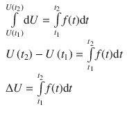
We consider a quantity U which changes over time t ; U is then a function of t and denoted as U ( t ).
At time t 1 ( start ): U = U ( t 1 )
At time t 2 ( end ): U = U ( t 2 )
The difference in U at times t 1 and t 2 (Fig. A.1a ) is indicated as Δ U (differences are always calculated as end minus start ):
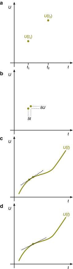
Fig. A.1
Graphical illustration of differences and differentials. For explanation see text
![]()
The slope of the line joining U ( t 2 ) and U ( t 1 ) is calculated as
The use of Δ to indicate a difference does not imply anything about the size of the difference. If we want to imply a very small change, we write δ U instead of Δ U (Fig. A.1b ).
We now consider U to be a continuous function of t as opposed to the discrete function with two individual points as above (Fig. A.1c ).
Now consider two time points t 1 and t 2 very close to each other, such that the difference between the two is infinitesimal (infinitely small). The line passing through the two points U ( t 2 ) and U ( t 1 ) is now called the tangent of U at point t 1 (Fig. A.1d ).
The slope of the tangent is still Δ U /Δ t , but because Δ t is now infinitesimal small, we use ’d’ instead of ’Δ’:
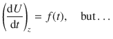
d U /d t tells us how U is varying with t at a particular point.
The lower case ’d’ indicates that the changes in t (and normally U ) are infinitesimal. There are various functions f for which the derivative is known analytically, e.g. f ( x ) = ln x => d f ( x )/d x = x −1 .
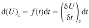
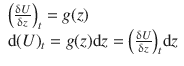
If we are told that

then a small change in t will result in a small change in U :
![]()
d U is called the differential of U . ![]() is called the Leibniz notation; another notation may be U ′( t ).
is called the Leibniz notation; another notation may be U ′( t ).
You can integrate both sides of this equation to get the overall change in U as the system changes from its initial to its final state:
A.2.2 Functions of More Than One Variable
Consider we have a function that varies with two variables, z and t (see Fig. A.2 ) ; we denote this as U ( z , t ).
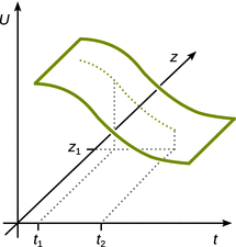
Fig. A.2
Variation of a function U in dependence of two parameters, t and z
How does U change with t when z is fixed? This may be denoted as:
we replace ![]() with
with ![]() (which is called the partial derivative) to indicate that U is a function of more than one variable:
(which is called the partial derivative) to indicate that U is a function of more than one variable:

So if z is fixed:
Similarly, we can now look at how U changes with z when t is fixed:
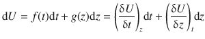
Therefore, the total differential of U when both variables, t and z , are allowed to vary is given by:
A.2.3 Product Rule
The product rule is a formula used to find the derivatives of products of two or more functions.
Consider the function h being the product of two functions, f and g :
![]()
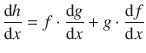
The derivative of h is then calculated according to the product rule:
![]()
which can be written in the Leibniz notation:
or, after multiplying with d x on both sides:
![]()
A.2.4 Functions with Known Derivatives
Table A.1
Functions with known derivatives
|
Function |
Derivative |
f ( x ) = a ; a = const. |
f ′( x ) = d f ( x )/d x = 0 |
f ( x ) = x |
f ′( x ) = d f ( x )/d x = 1 |
f ( x ) = x n |
f ′( x ) = d f ( x )/d x = n · x n −1 |
f ( x ) = 1/ x = x −1 |
f ′( x ) = d f ( x )/d x = −1/ x 2 = − x −2 |
f ( x ) = 1/ x n = x − n |
f ′( x ) = d f ( x )/d x = − n / x n +1 = − n·x − n −1 |
f ( x ) = |
f ′( x ) = d f ( x )/d x = 1/ n · x n −1 |
f ( x ) = e x |
f ′( x ) = d f ( x )/d x = e x |
f(x) = a x ; a = const. |
f ′( x ) = d f ( x )/d x = a x ·ln a |
f(x) = ln x |
f ′( x ) = d f ( x )/d x = 1/ x = x −1 |
f ( x ) = sin x |
f ′( x ) = d f ( x )/d x = cos x |
f ( x ) = cos x |
f ′( x ) = d f ( x )/d x = −sin x |
A.3 Integration
Integrating is similar to summing a property as is it gradually changes from one state to another. Therefore, U is simply the sum of all the infinitesimal changes d U .
There are various functions f for which the integral is known analytically. You may remember a number of these (e.g. ∫ x −1 d x = ln x ).
A.3.1 Functions with Known Integrals
Table A.2
Functions with known integrals
|
Function |
Integral |
f ( x ) = a ; a = const. |
∫ f ( x ) d x = ∫ a d x = a ·∫ d x = a · x |
f ( x ) = x |
∫ f ( x ) d x = ∫ x d x = 1 / 2 x 2 |
f ( x ) = x n |
∫ f ( x ) d x = ∫ x n d x = 1/( n +1) x n +1 |
f ( x ) = 1/ x = x −1 |
∫ f ( x ) d x = ∫ 1/ x d x = ln | x |; x ≠ 0 |
f ( x ) = 1/ x n = x − n |
∫ f ( x ) d x = ∫ x − n d x = 1/(‑ n +1) x ‑ n +1 ; n ≠ 1 |
f ( x ) = |
∫ f ( x ) d x = ∫ x 1/ n d x = 1/(1/ n +1) x 1/ n +1 |
f ( x ) = e x |
∫ f ( x ) d x = ∫ e x d x = e x |
f ( x ) = e ax |
∫ f ( x ) d x = ∫ e ax d x = 1/ a ·e x |
f(x) = a x ; a = const. |
∫ f ( x ) d x = ∫ a x d x = a x /(ln a ) |
f ( x ) = ln x |
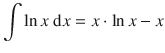
∫(ln x ) d x = x ⋅ ln x − x |
f ( x ) = sin x |
∫(sin x ) d x = − cos x |
f ( x ) = cos x |
∫(cos x ) d x = sin x |
f ( x ) = sin 2 ( a ⋅ x ) |
|
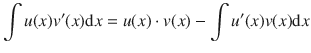
A.3.2 Rule for Partial Integration
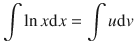
The rule for partial integration is useful for integration of more complicated functions. In particular, the rule relates the integral of a product of two functions, ∫ u ( x ) v ′( x ), to the integral of their derivative and anti-derivative, ∫ u ′( x ) v ( x )d x . It is frequently used to transform the anti-derivative of a product of functions into an anti-derivative for which a solution can be more easily found.
Example: Integrate the function ln x .

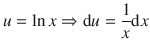
This can be solved by using partial integration. Define two appropriate functions u and v :
![]()
Therefore:
We know the derivative of u :
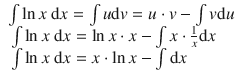
The anti-derivative of d v is v , therefore:
![]()
So we can now solve the substituted integral:
With ∫d x = x this yields:
A.4 Data Visualisation and Fitting
A.4.1 Software
Very commonly, basic data visualisation and analysis (such as averaging, error estimation and fitting with linear functions) can be carried out with generic spreadsheet programs such as MS Excel or the spreadsheet programs from the open-source suites LibreOffice or OpenOffice . More sophisticated software dedicated to data analysis and visualisation include the commercial products SigmaPlot , Origin , Prism , IGOR and others. There are also free and open-source programs (see Table A.3 ).
Table A.3
Some free and open-source software for data analysis and visualisation
|
Software |
Web page |
Reference |
R |
http://www.R-project.org/ |
|
SDAR |
http://www.structuralchemistry.org/pcsb/sdar.php |
Weeratunga et al. ( 2012 ) |
Grace |
http://plasma-gate.weizmann.ac.il/Grace/ |
|
gnu-plot |
http://www.gnuplot.info/ |
|
Fityk |
Wojdr ( 2010 ) |
|
peak-o-mat |
http://lorentz.sourceforge.net / |
|
HippoDraw |
http://www.slac.stanford.edu/grp/ek/hippodraw/ |
|
Veusz |
http://home.gna.org/veusz/ |
|
ParaView |
http://www.paraview.org / |
A.4.2 Independent and Technical Repeats
Measurements are repeated in order to obtain estimates of the precision of the experimental method. Repeating the measurement of an individual sample several times does not constitute an independent repeat; rather, it is a technical repeat. In order to obtain independent repeats, the same condition needs to be reproduced multiple times. A commonly used parameter to assess precision is the estimated standard deviation σ exp :
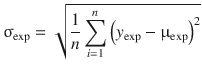
where ![]() is the mean of the experimental values.
is the mean of the experimental values.
A.4.3 Data Visualisation
The way data are presented can make a substantial difference to the perception of experimental results by the reader. A typical example is the scale chosen; the plot of a baseline can be presented as a steady straight line or as noisy data, depending on the scale of the y -axis. Other aspects to consider are the type of plot used (line graphs, bar graphs, pie charts, etc).
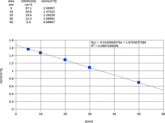
Fig. A.3
Example plot of experimental data with superimposed linear fit using the free spreadsheet software LibreOffice
Here, we will focus on some basic considerations for simple two-dimensional plotting of data. In general, the following should be followed (Fig. A.3 ):
✵ Plots are presented with respect to two dimensions, one on the x -, the other on the y -axis. Always label the axes with the parameter that is plotted in that dimension; include the units. For example: x -axis: c (NaOH) in mM; y -axis: A(280 nm)—no units, since absorbance is a scalar.
✵ The scale needs to be available to the reader. This means that in most cases one needs to indicate the origin of each axis (’0’) and at least one data point (e.g. ’1 mM’).
✵ Choose appropriate scales on the axes, and avoid overly long numbers. For example, instead of ’0.0001 M, 0.0002 M, …’ label ticks with ’0.1 mM, 0.2 mM, …’.
✵ If an experiment comprised of acquisition of individual data points (e.g. absorbance of a sample at select concentrations of a reactant), then the data are discrete data points and should be plotted as individual points, without connecting them with lines; this is called a scatter plot. Only if (quasi-) continuous data have been acquired (e.g. by using sensor readings at a reasonably high sampling rate), the data can be shown as line graphs. In a line plot, individual data points may or may not be visible and subsequent data points are connected by a line.
✵ If independently repeated measurements for individual conditions are available, the values for each condition are averaged and the estimated standard deviation is calculated. Error bars are constructed by adding and subtracting the estimated standard deviation to/from the averaged value.
✵ Discrete data (scatter plots) are never smoothed; only (quasi-)continuous data may be subjected to smoothing procedures.
✵ Data fitting may be undertaken as a means to show agreement with a theoretical model. Data fits are superimposed on the experimental data as line plots. Since data fits arise from a theoretical model with a numerical equation, they are per definition continuous data.
A.4.4 Data Fitting
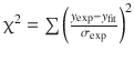
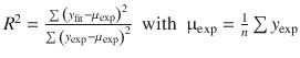
When fitting a theoretical model to experimental data, statistical parameters need to be calculated to assess the goodness of fit between the theoretical and experimental data. Commonly used statistical parameters include:
In Table A.4 , μ exp is the mean and σ exp the estimated standard deviation of the experimental data. The parameter χ 2 is a weighted measure of error, since it is divided by the estimated standard deviation (i.e. the error appearing in independent repeats); the non-weighted χ 2 is identical to the summed square error.
Table A.4
Commonly used goodness-of-fit parameters
|
Parameter |
Definition |
Value for perfect fit |
Chi-square |
|
0 |
R -square |
|
1 |
Summed square error |
SSE = ∑ ( y exp − y fit ) 2 |
0 |
R -factor |
|
0 |
A.4.5 Correlation
In order to evaluate the correlation of two different quantities (e.g. the variables x and y ), correlation coefficients can be determined.
The Pearson product-moment correlation coefficient r is a measure of the linear correlation between two variables x and y , giving a value between +1 and −1:
✵ +1: total positive correlation
✵ 0: no correlation
✵ −1: total negative correlation
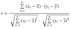
Here, ![]() and
and ![]() denote the arithmetic mean over all x - and y -values, respectively.
denote the arithmetic mean over all x - and y -values, respectively.
If the two variables x and y are related in a monotonous fashion, but a linear relationship cannot be expected, then Spearman’s rank correlation coefficient instead of the Pearson correlation needs to be applied.