Physical Chemistry Essentials - Hofmann A. 2018
Appendix B Solutions to Exercises
Chapter 2
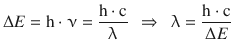
2.1. Calculate the work done per mole when an ideal gas is expanded reversibly by a factor of 3 at 120 °C.
![]()
The work is done by the system (hence we count it as negative) in a reversible process from state ’1’ at the volume V start = V 1 to state ’2’ at volume V end = 3· V 1 . In order to obtain the amount work during the entire process, we need to integrate above equation:
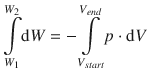
During the reversible process, the outside pressure is constantly adjusted to match the pressure in the system. Hence, p is a function V and calculated as per the ideal gas equation:

Therefore:
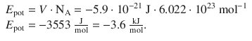
The work done when 1 mol of an ideal gas is expanded reversibly by a factor of 3 at 120 °C is −3.6 kJ.
2.2. A friend thinking of investing in a company that makes engines shows you the company’s prospectus. Analysing the machine, you realise that it works by harnessing the expansion of a gas. The operating temperature is approx. constant at 120 °C, and the gas doubles in volume during the power extraction phase of operation. It is claimed that the machine produces 5.5 kJ mol −1 of work during expansion. What advice would you give your friend? Briefly explain the thermodynamic rationale.
No process can produce more work than an equivalent process (see Exercise 2.1) running under reversible conditions. The claim that the machine produced 5.5 kJ mol −1 is thus in error. Your friend should not invest.
2.3. Which of the following equations embodies the first law of thermodynamics:
1. (a)
2. (b)
3. (c)
4. (d)
5. (e)
In the integrated form, the first law of thermodynamics states that the internal energy of a system ( U ) comprises of heat ( Q ) and work ( W ); the correct answer is therefore (b). (a) is the definition of entropy change of a system for a reversible process; (c) describes the second, and (d) the third law of thermodynamics; (e) is the definition of the heat capacity for processes under constant pressure.
2.4. If the pressure is constant, the system is in mechanical equilibrium with its surroundings and no work is done other than work due to expansion and compression, which of the following are true:
1. (a)
2. (b)
3. (c)
4. (d)
5. (e)
The correct answer is (a). Under constant external pressure the enthalpy change equals the transferred heat if only work due to expansion and compression is done.
In solution (c), ’Δ U = Δ Q − p ·Δ V ’ is correct, but ’Δ W = p ·Δ V ’ is not correct!
2.5. Which of the following equations define fugacity?
1. (a)
2. (b)
3. (c)
The correct answer is (a). The fugacity replaces the pressure in the equation for the chemical potential to account for non-ideal behaviour of gases. Fugacity measures how compressible a gas is compared to the ideal gas; it is measured in units of pressure. Therefore, (b) is not correct, as this would yield a scalar. (c) describes the chemical equation for a solution containing a solute A of activity a .
2.6. The chemical potential is defined as:
1. (a)
2. (b)
3. (c)
4. (d)
5. (e)
6. (f)
The correct answers are (b) and (f). The chemical potential is defined as the molar free energy, i.e. the free energy of 1 mol of substance. Note that (e) is not correct, as these are not molar free energies.
Chapter 3
3.1. Is it possible for a one-component system to exhibit a quadruple point?
For a one-component system ( C = 1) to exhibit a quadruple point ( P = 4), the Gibbs phase rule yields F = C — P + 2 = 1—4 + 2 = −1. Since the number of degrees of freedom cannot be negative, a quadruple point cannot exist in a one-component system.
3.2. Henry’s law is valid for dilute solutions. Using the Henry’s law constant for oxygen (solute) and water (solvent) of K (O 2 ) = 781·10 5 Pa M −1 , calculate the molar concentration of oxygen in water at sea level with an atmospheric pressure of p atm = p — .
Since the fraction of O 2 in the atmosphere is 21%, its partial pressure is p (O 2 ) = 0.21· p atm = 0.21·p — = 0.21·10 5 Pa. From Henry’s law, this yields c (O 2 ) = 0.27 μM.
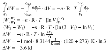
3.3. Below is the T - x phase diagram of the benzene/toluene system acquired at a constant pressure of two bar. A mixture that contains 40% benzene is heated steadily to 122 °C. How many phases are present at this point and what are their compositions? If the total amount of 1 mol of substances was in the initial mixture with 40% benzene, how many moles of substances are in the phase(s) at 122 °C?
At 122 °C (395 K), there are two phases: x liq (benzene) = 0.34, x vap (benzene) = 0.54. According to the lever rule, the ratio of molar amounts in the liquid and vapour phase is ![]() . Since the total amount of substances in the mixture was set at n 0 = 1 mol, there is n liq = 0.72 mol and n vap = 0.28 mol.
. Since the total amount of substances in the mixture was set at n 0 = 1 mol, there is n liq = 0.72 mol and n vap = 0.28 mol.
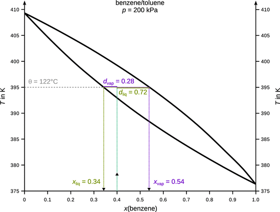
3.4. A mixture of benzene and toluene with x(benzene) = 0.4 is subjected to fractional distillation at two bar (see Exercise 3.3 above). What is the boiling temperature of this mixture? How many theoretical plates are required as a minimum to obtain pure benzene in the distillate?
The mixture boils at 393 K (120 °C). A minimum of five theoretical plates are required to obtain pure benzene.
Chapter 4
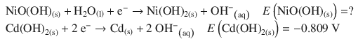
4.1. Nickel-cadmium batteries are based on the following half-cell reactions:
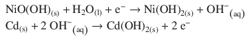
1. (a)
✵ The half-reactions for the nickel cadmium cell are:
✵ In order for the nickel-cadmium cell to operate, the second reaction needs to run in reverse, i.e. it constitutes the oxidation; the first reaction constitutes the reduction.
1. (b)
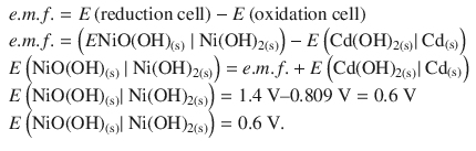
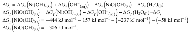
✵ The standard Gibbs free energy change for the overall nickel half-cell reaction can be calculated as per:
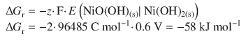
✵ The standard Gibbs free energy of formation is then obtained from the reaction free energy:
4.2. Calculate the standard e.m.f. and the equilibrium constant under standard conditions for the following cell:
![]()
This cell consists of the following two half-cells:
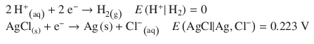
According to the reduction potentials, the first reaction needs to run as oxidation, and the second one as reduction, just like the electrochemical notation suggests. The standard e.m.f. is then calculated as per:
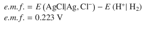
The net reaction in the electrochemical cell is thus:
![]()
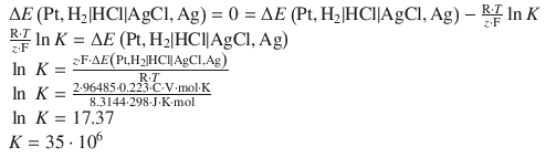
When this reaction is in equilibrium, there is no potential difference between the two half cells:
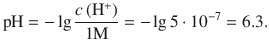
4.3. Calculate the pH of a solution with a formal concentration of 5·10 −7 M of the strong acid HI at 25 °C.
Strong acids fully dissociate in aqueous solution:
![]()
Therefore, the concentration of protons and base anion is:
![]()
The pH can thus be calculated as:
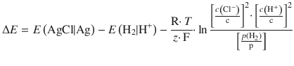
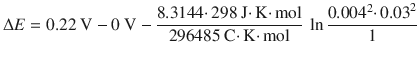
4.4. What e.m.f. would be generated by the following cell at 25 °C, assuming ideal behaviour:
![]()
This cell consists of the following two half-cells:
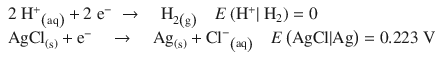
According to the reduction potentials, the first reaction needs to run as oxidation, and the second one as reduction, just like the electrochemical notation suggests. The net reaction in the electrochemical cell is thus:
![]()
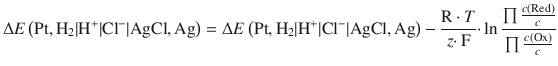
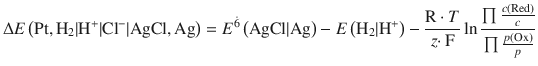
The concentration dependence of an electrochemical cell is given by the Nernst equation:
![]()
![]()
![]()
The e.m.f. generated is 0.46 V.
4.5. The lactate/pyruvate Redox system can be described as per:
![]()
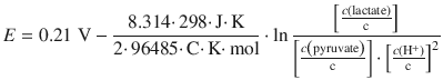
The standard reduction potential is measured at c (lactate) = c (pyruvate) = c (H + ) = 1 M and has a value of E — = 0.21 V. Calculate and plot the pH dependency of the reduction potential for this system at 298 K, assuming c (lactate) = c (pyruvate).
The concentration dependence is given by the Nernst equation:
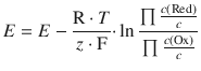
where c (Ox) refers to the concentration on the oxidised side and c (Red) to the concentrations on the reduced side of the equilibrium reaction. Therefore:
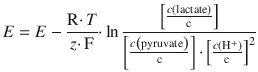
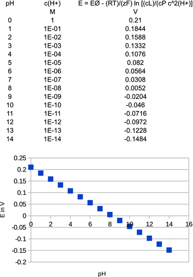
The relationship between the reduction potential and the pH is linear with E (pH = 0) = 0.21 V and E (pH = 14) = −0.15 V, i.e. a slope of −0.026 V per pH unit.
Chapter 5
5.1. At 25 °C, the molar ionic conductivities Λ m of alkali ions are
Table B.1
Molar conductivities for select alkali ions
|
Ion |
Λ m (mS m 2 mol −1 ) |
Li + |
3.87 |
Na + |
5.01 |
K + |
7.35 |
What are their mobilities?
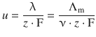
The mobility of ions provides a link between their charge and the conductivity in solution:
![]()
The molar conductivity Λ m is linked to the conductivity λ of the counter-ions by:
![]()
Since we are interested in the isolated alkali ions, we set Λ m = ν + ·λ + with ν + = 1.
Therefore:
For Li + , this yields:
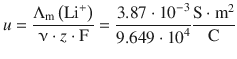
Remember that 1 S = 1 Ω −1 = 1 A/V, and that 1 C = 1 A s. Therefore:
In summary:
Table B.2
Ion mobilities for select alkali ions
|
Ion |
Λ m (mS m 2 mol −1 ) |
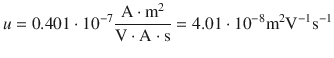
u (m 2 V −1 s −1 ) |
Li + |
3.87 |
4.01·10 −8 |
Na + |
5.01 |
5.19·10 −8 |
K + |
7.35 |
7.62·10 −8 |
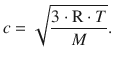
5.2. Fullerene (C 60 ) has a diameter of 10.2 Å. Estimate the diffusion coefficient of fullerene in benzonitrile at 25 °C. The viscosity of benzonitrile at that temperature is 12.4 mP. How large is the error of your estimate when comparing the result to the experimental value of 4.1·10 −10 m 2 s −1 ?
The diffusion coefficient can be calculate by the Stokes-Einstein relationship:
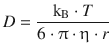
The viscosity is η(benzonitrile) = 12.4 mP = 12.4·10 −3 P = 1.24·10 −3 N s m −2
The radius is r (C 60 ) = 1 / 2 ·10.2 Å = 5.1 Å = 5.1·10 −10 m
Therefore:
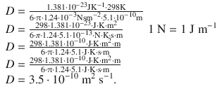
The calculated diffusion coefficient thus has a value of 3.5·10 −10 m 2 s −1 . The difference to the experimental value is:
![]()
This is an error of approximately
The relatively large error is due to the very nature of the Stokes-Einstein relationship which applies thermodynamic quantities (temperature, the average energy of particles k B · T ) that relate to large numbers of particles to single molecules.
5.3. The mean free path length of gas molecules can be calculated according to Maxwell as ![]() , where the particle density is
, where the particle density is ![]() . Calculate the diffusion coefficient of argon at 298 K and a pressure of 1 bar. The collisional cross-section of argon is σ = 0.41 nm 2 .
. Calculate the diffusion coefficient of argon at 298 K and a pressure of 1 bar. The collisional cross-section of argon is σ = 0.41 nm 2 .
The diffusion coefficient for an ideal gas is calculated as per

The mean speed of molecules, c , is calculated as per
The mean free path length is accessible from above formulae as per
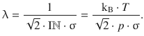
This yields for the diffusion coefficient:
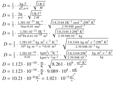
The diffusion coefficient of argon thus has a value of 1.021·10 −5 m 2 s −1 .
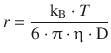
5.4. The diffusion coefficient of sucrose in water is 5.2·10 −6 cm 2 s −1 at room temperature. Estimate the effective radius of a sucrose molecule, if water has a viscosity of 10 mP.
The diffusion coefficient can be calculate by the Stokes-Einstein relationship:
The effective radius of the molecule is then:
The viscosity is η(water) = 10 mP = 1.0·10 −2 P = 1.0·10 −3 N s m −2
The diffusion coefficient is D (sucrose) = 5.2·10 −6 cm 2 s −1 = 5.2·10 −10 m 2 s −1 .
Therefore:
The effective radius of a sucrose molecule is thus estimated at 4.2 Å.
Chapter 6
6.1. Consider the gas-phase reaction
![]()
1. (a)
✵ If the reaction order is as suggested by the chemical equation, we are dealing with first order kinetics:
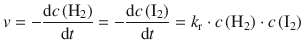
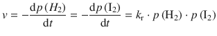
✵ Since this is a gas phase reaction, and all parameters are given in the units of pressure, we can substitute the molar concentration against the pressure:
✵ The data given are:
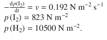
✵ Therefore
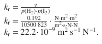
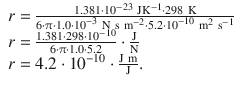
✵ To obtain the rate constant in molar units, we assume ideal gas conditions, and thus ![]()
✵ k r = 22.2·10 −9 m 2 s −1 N −1 ·8.3144 J K −1 mol −1 ·681 K
✵ k r = 0.126·10 −3 m 3 s −1 mol −1
✵ k r = 0.126 M −1 s −1 .
1. (b)
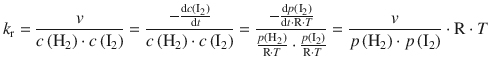
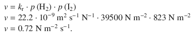
✵ The rate of the reaction for the new hydrogen pressure p (H 2 ) = 39500 N m −2 is then
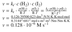
✵ Alternatively, if we calculate the rate in molar units instead of pressure:
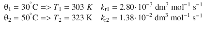
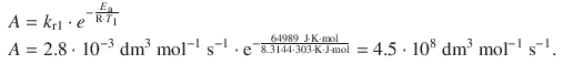
6.2. The rate constant for the decomposition of a particular substance is 2.80·10 −3 dm 3 mol −1 s −1 at 30 °C, and 1.38·10 −2 dm 3 mol −1 s −1 at 50 °C. Evaluate the Arrhenius parameters of the reaction.
Data compilation:
As above, we build the ratio of the two Arrhenius equations for the two conditions:
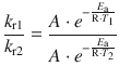
and obtain after cancellation of the pre-exponential parameter A and some re-arrangements:
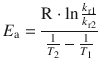
This yields for the data given:
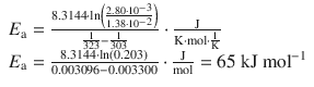
This allows calculation of the pre-exponential factor:
6.3. The reaction mechanism for the reaction of A 2 and B to product P involves the intermediate A:
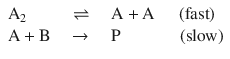
Deduce the rate law for the reaction assuming a pre-equilibrium.
If we assume an equilibrium for the first reaction, we know that the equilibrium constant K is the ration of the rate of the forward ( k 1 ) and reverse reaction ( k −1 ). We also know that this equals the ratio of the equilibrium concentrations of A 2 and A:
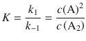
This yields for the equilibrium concentration of A:
![]()
For the second reaction, the rate equation is:
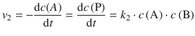
Substituting the expression for the equilibrium concentration of A yields:
![]()
6.4. The rate constant of a first-order reaction was measured as 1.11·10 −3 s −1 .
1. (a)
✵ The first order rate law is
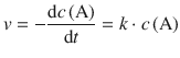
✵ and the half-life is

✵ Therefore:
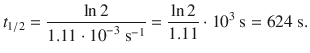
1. (b)
✵ In order to calculate a different life time, the differential rate law needs to be integrated:
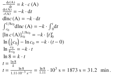
1. (c)
✵ In analogy to the above, one derives:
Chapter 7
7.1. The initial rates of the myosin-catalysed hydrolysis of ATP were measured in the presence of varying starting concentrations of ATP:
Table B.3
Initial rates for myosin-catalysed ATP hydrolysis
c 0 (ATP) |
mmol dm −3 |
0.005 |
0.010 |
0.020 |
0.030 |
0.050 |
0.100 |
0.200 |
0.300 |
v 0 |
μmol dm −3 s −1 |
0.051 |
0.083 |
0.118 |
0.138 |
0.158 |
0.178 |
0.190 |
0.194 |
Assume that the enzymatic reaction follows a Michaelis-Menten mechanism and determine the maximum rate and the Michaelis constant.
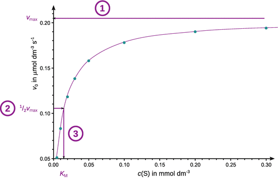
For an accurate determination of v max , the original data either need to be fitted with by non-linear regression (above) or transformed into a reciprocal relationship that linearises the Michaelis-Menten equation, e.g. by using the Lineweaver-Burk approach:
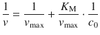
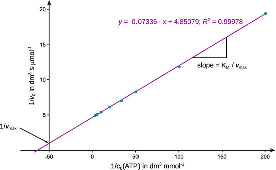
Table B.4
Lineweaver-Burk transformation of the initial data
1/ c 0 (ATP) |
dm 3 mmol −1 |
200 |
100 |
50.0 |
33.3 |
20.0 |
10.0 |
5.00 |
3.33 |
1/ v 0 |
dm 3 s μmol −1 |
19.6 |
12.1 |
8.47 |
7.25 |
6.33 |
5.62 |
5.26 |
5.15 |
The fit with a linear equation yields a function:

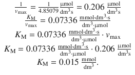
From the line fit one obtains:
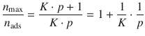
7.2. The adsorption behaviour of 1 g activated carbon at 0 °C has been quantitatively assessed using different pressures of N 2 . The following molar amounts of N 2 are adsorbed:
Table B.5
Data for adsorption of N 2 by activated carbon
p (N 2 ) |
kPa |
0.524 |
1.73 |
3.06 |
4.13 |
7.50 |
10.3 |
n ads (N 2 ) |
10 −4 mol |
0.440 |
1.35 |
2.27 |
3.14 |
4.60 |
5.82 |
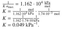
Assuming Langmuir adsorption behaviour, determine (a) the maximum amount of N 2 that can be adsorbed by 1 g activated carbon at 0 °C, and (b) the Langmuir constant.
The Langmuir adsorption isotherm is
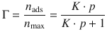
Taking the reciprocal value on both side of above equation yields:
and thus
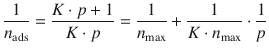
From this equation, it is obvious that a plot of 1/ n ads versus 1/ p yields a line with y -intercept 1/ n max and slope 1/( K · n max ).
The reciprocal values of the original data yield:
Table B.6
Transformation of initial data for Langmuir adsorption isotherm
1/ p (N 2 ) |
kPa −1 |
1.91 |
0.578 |
0.327 |
0.242 |
0.133 |
0.0968 |
1/ n ads (N 2 ) |
10 4 mol −1 |
2.27 |
0.741 |
0.441 |
0.318 |
0.217 |
0.172 |
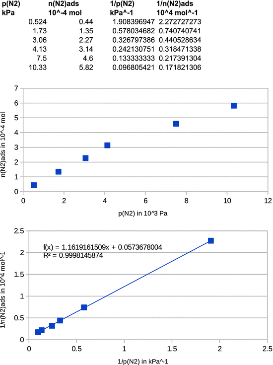
Linear fit of these data result in the following equation:
![]()
1. (a)
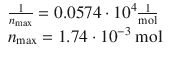
1. (b)
Chapter 8
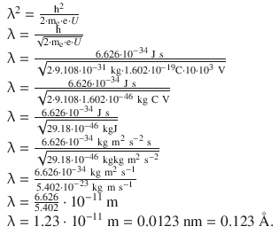
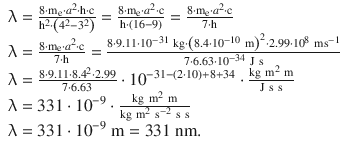
8.1. Calculate the wavelength of an electron that is accelerated by a potential difference of 10.0 kV.
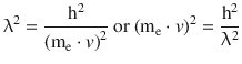
The energy gained by an electron accelerated in an electric field (its kinetic energy) equals the potential energy provided by the electric field:
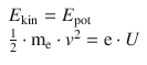
The DeBroglie relationship links the wave and corpuscular properties of a particle in form of the wavelength λ and the momentum p. Specifically for the electron, this yields:
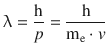
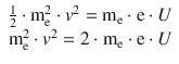
The squared equation yields:
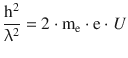
We now multiply me into both sides of above energy equation and obtain:
For the squared momentum we can substitute the wavelength expression from the DeBroglie relationship:
Resolving for the wavelength yields:
8.2. The atomic model suggested by Niels Bohr in 1913 depicts atoms as systems very much like a solar system, where electrons travel in circular orbits around the positively charged nucleus. If one wanted to determine the location of an electron at a particular point in time with a certainty of ±0.05 Å, what is the uncertainty with respect to the speed of the electron?
The uncertainty relationship by Heisenberg informs of the minimum value of the product (Δ x ·Δ p ):
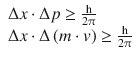
With m = m e and Δ x = 0.1 Å, this yields:
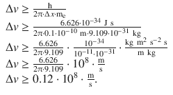
The uncertainty about the speed of the orbiting electron is approx. 0.12·10 8 m s −1 . This dramatically high uncertainty shows that no statement as to the exact location of the electron can be made at a particular time.
8.3. The wavelength of macroscopic objects. What is the wavelength of a person of 65 kg walking at a speed of 0.8 m s −1 ?
According to the deBroglie relationship, the wavelength λ is related to the momentum of an object as per:
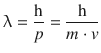
This yields:
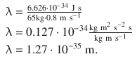
This is a very tiny wavelength; for comparison, the proton has a radius of about 0.8 fm = 0.8·10 −15 m. This explains why the waves of macroscopic objects cannot be measured.
8.4. Two consecutive lines in the atomic spectrum of hydrogen have the wave numbers ν˜ i = 2.057·10 6 m −1 and ν˜ i +1 = 2.304·10 6 m −1 . Calculate to which series these two transitions belong and which transitions they describe.
According to Bohr’s term scheme, the wave numbers for the two transitions are related to the states n 0 , n i and n i +1 as per:
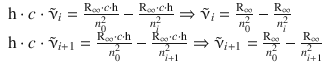
Subtraction of the first equation from the second yields:
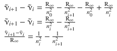
The left hand side of this equation computes as per:
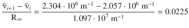
From comparison of this value with the following transitions between n i and n i +1 we find a suitable pair n i , n i +1 :
Table B.7
Term scheme differences
|
n i |
n i + 1 |
|
|
|
|
|
1 |
2 |
1 |
0.5 |
1 |
0.25 |
0.75 |
2 |
3 |
0.5 |
0.3333 |
0.25 |
0.1111 |
0.1389 |
3 |
4 |
0.3333 |
0.25 |
0.1111 |
0.0625 |
0.0486 |
4 |
5 |
0.25 |
0.2 |
0.0625 |
0.04 |
0.0225 |
5 |
6 |
0.2 |
0.1667 |
0.04 |
0.0278 |
0.0122 |
![]()
With this knowledge, we can calculate n 0 :
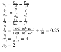
The two transitions thus are: n 0 = 2 → n = 4 and n 0 = 2 → n = 5. Since n 0 = 2, the transitions belong to the Balmer series.
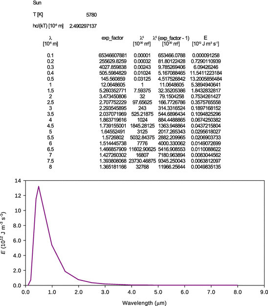
8.5. Assuming that (a) the sun ( T = 5780 K) and (b) the earth ( T = 298 K) behave as black-bodies, calculate and plot the spectral flux densities for the sun and the earth. What are the similarities and differences between both radiation curves? Use Planck’s law to calculate E (λ) for the wavelength range 100 nm—8 μm. Calculation and plotting might be best done with a spreadsheet software.
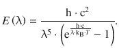
Planck’s law describes radiation (spectral flux density) E (λ) of a black-body at varying wavelengths for a a particular temperature:
We set out to calculate E (λ) for the following wavelengths in a spreadsheet program:
Table B.8
Wavelength values in μm
0.1 |
0.2 |
0.3 |
0.4 |
0.5 |
1.0 |
1.5 |
2.0 |
2.5 |
3.0 |
3.5 |
4.0 |
4.5 |
5.0 |
5.5 |
6.0 |
6.5 |
7.0 |
7.5 |
8.0 |
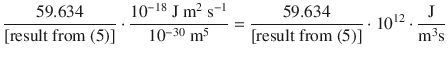
Since above equation involves several factors with large exponential values, we separate the problem into different individual steps and deal with the exponential factors manually, since such software use floating point numbers, which is a finite sized representation. Therefore, approximated results or error conditions might occur when using very large numbers.
1. (1)
2. (2)
3. (3)
4. (4)
Table B.9
The four quantum numbers of the electron
|
Name |
Symbol |
Values |
Description |
Principal quantum number |
n |
0, 1, 2, ... |
Size of the wave function, energy level. |
Angular momentum quantum number |
l |
0, 1, ..., ( n −1) |
Shape of the wave function. |
Magnetic quantum number |
m l |
− l , (− l +1), ..., 0, ..., ( l −1), l |
Orientation of the wave function in space. |
Magnetic spin quantum number |
m s |
− 1 / 2 , + 1 / 2 |
Orientation of the magnetic moment of the electron. |
![]()
1. (5)
2. (6)
1. (a)
1. (b)
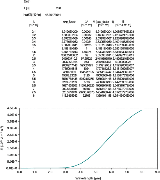
From comparison of both radiation curves, we see that the earth emits less radiation than the sun (note the difference of orders of magnitude on the y -axes). Also, the interesting wavelength range is 0.4—0.7 μm (or 400—700 nm), as this is the visual range. Whereas the earth as a comparably cold planet emits no radiation in the visual range, this is different for hot stars such as the sun. The maximum of the spectral flux density for the sun is exactly in the range of visual light.
Chapter 9
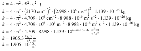
9.1. The radius of the first orbit in the Bohr model is r 1 = 5.3·10 −9 cm. As a rough estimate, calculate the energy of the electron in the hydrogen atom, assuming it was a particle in a cubic box of the same volume as that of a sphere with radius r 1 . Compare the result with the energy that is predicted by the Bohr model.
1. (1)
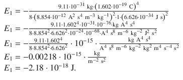
✵ The energy of the electron in different orbits is given by
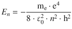
for n = 1 this yields:
1. (2)
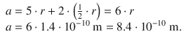
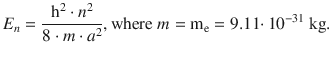
✵ The energy of a particle in a three-dimensional box is given by
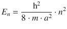
✵ Since we assume a cubic box where the volume equals the volume of a sphere with the radius of the first orbit in the Bohr model, we can calculate a as follows:
✵ We can now calculate the energy of the particle in a cubic box of width a with n = 1:
Comparison of the numerical values of the energies for the first orbit in the Bohr model with the lowest energy state in the quantum mechanical model shows that the energy predicted by the Bohr model is by an order of magnitude lower.
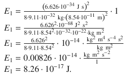
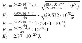
9.2. Calculate the zero-point energy of 1 H 35 Cl (a) for one molecule, and (b) for 1 mol, assuming a force constant of 480.6 Nm −1 .
The zero-point energy is given by
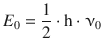
where ν 0 is the frequency of vibrational oscillation of a di-atomic molecule defined by
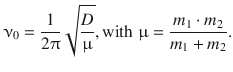
Therefore:
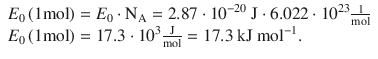
For 1 mol of HCl, one needs to multiply with Avogadro’s constant:
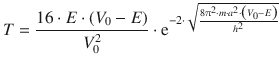
9.3. What is the value of the transmission coefficient for an electron with an energy of 1 eV that moves against a potential barrier of 5 eV and 2 nm thickness?
The transmission coefficient is given by
With m = m e = 9.110·10 −31 kg, one obtains:
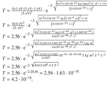
The transition coefficient is 4.2·10 −18 .
9.4. Calculate the probability of locating a particle in a potential-free one-dimensional box of length a between 1 / 4 a and 3 / 4 a , assuming the particle being in its lowest energy state.
The probability of finding the particle is described the squared wave function |Ψ| 2 . The normalised wave function solving the Schrödinger equation for a one-dimensional box without a potential is given by
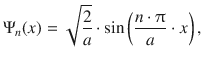
which yields for the probability:
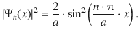
In order to calculate the probability density, the accumulated probability to find the particle between 1 / 4 a and 3 / 4 a , the probability needs to be integrated in this region:
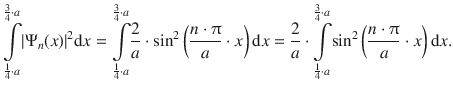
We find that we need to integrate a function of the type sin 2 ( C ⋅ x ), with ![]() for which the following integral is known:
for which the following integral is known:
With n = 1 (lowest energy state), this yields:
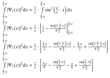
The probability to find the particle between 1 / 4 a and 3 / 4 a is 82%.
Chapter 10
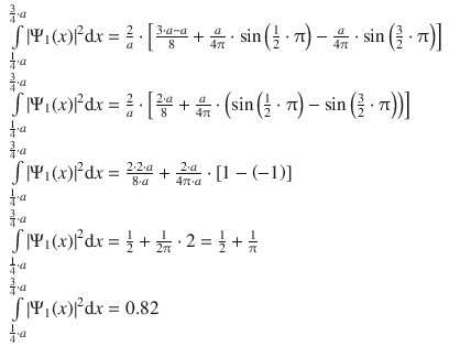
10.1. Calculate at which distances from the nucleus the 3 s orbital possesses radial nodes.
The radial eigenfunction for the 3 s orbital ( n = 3, l = 0) is
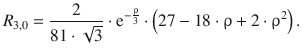
Nodes are areas in which the probability to find the electron is zero. For the 3 s orbital, the number of radial nodes is ( n — l —1) = (3—0—1) = 2. In the eigenfunction, these are the points where the function has a zero-crossing, i.e. the function assumes a value of zero. Therefore:
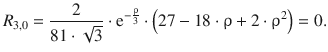
This function is a product of three factors; neither the scalar factor ![]() nor the exponential factor
nor the exponential factor ![]() can assume a value of zero. The only factor that can assume a value of zero is the expression in brackets:
can assume a value of zero. The only factor that can assume a value of zero is the expression in brackets:
![]()
This is a quadratic equation; the zero-crossings are thus calculated as per the formula ![]() . This yields:
. This yields:
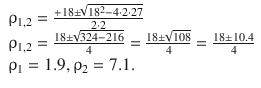
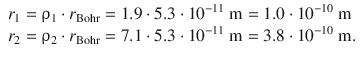
Since ρ is the ratio between a a radial distance and the radius of the first orbit r Bohr ( ![]() ), the metric distances of the two nodes are:
), the metric distances of the two nodes are:
10.2. Derive the electron configuration for (a) vanadium, and (b) chromium in their ground states.
1. (a)
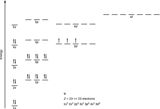
✵ The electronic configuration of vanadium is 1 s 2 2 s 2 2 p 6 3 s 2 3 p 6 3 d 3 4 s 2 .
1. (b)
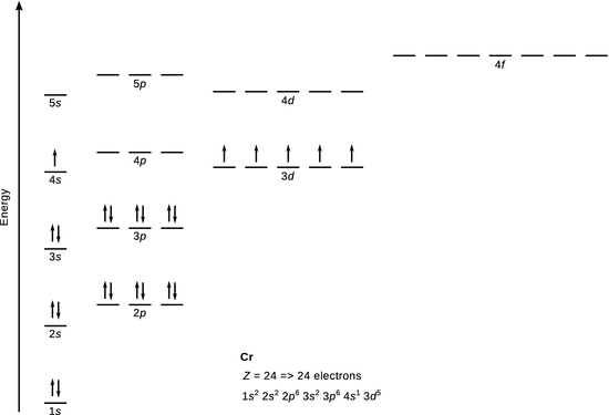
✵ The electronic configuration of chromium is 1 s 2 2 s 2 2 p 6 3 s 2 3 p 6 3 d 5 4 s 1 .
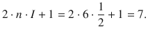
10.3. Name the four quantum numbers of the electron and state their relationships/possible values.
10.4. Describe the overall shape of the orbitals characterised by the angular momentum quantum number l = 0, 1, 2.
![]()
This is an s -orbital; it has spherical symmetry.
![]()
These are p -orbitals and they have a two-lobed structure.
![]()
These are d -orbitals; four of them adopt a four-lobed structure, one of them has rotational symmetry and consists of a two-lobed structure with a torus.
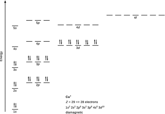
10.5. Determine the ground-state electronic configuration of the following species: S - , Zn 2+ , Cl − , Cu + .
S −
17 electrons
![]()
Zn 2+
28 electrons
![]()
Cl −
18 electrons
![]()
Cu +
28 electrons
![]()
10.6. a) Using the knowledge about the allowed energy states (eigenvalues), calculate the ionisation potential of the hydrogen atom.
The allowed energy states (eigenvalues) of the hydrogen atom are obtained as
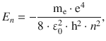
with n = 1, since the only electron in hydrogen in the ground state occupies the first shell. In order to remove the electron, the energy of | E 1 | needs to be provided, hence this is the ionisation energy.
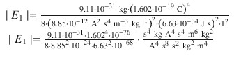
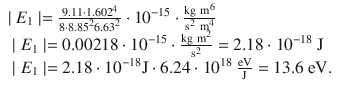
The ionisation energy of hydrogen is 13.6 eV.
b) The equation yielding the allowed energy states of a multi-electron atom is often modified to ![]() to accommodate the shielding of the nuclear charge by electrons in the various orbitals; the parameter σ is thus called the screening constant. Calculate the value of σ for helium, assuming its first ionisation potential is 24.5 eV.
to accommodate the shielding of the nuclear charge by electrons in the various orbitals; the parameter σ is thus called the screening constant. Calculate the value of σ for helium, assuming its first ionisation potential is 24.5 eV.
For non-hydrogen atoms ( Z > 1), the above equation for eigenvalues needs to consider the number of electrons (which equals the order number Z in the periodic system)
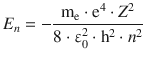
but then needs to be adjusted for the shielding of the nuclear charge by electrons present. One way to do this is to replace Z with ( Z −σ) where σ is called the screening constant:
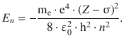
From the first ionisation energy of He (24.6 eV), the screening constant s can be calculated using the above equation. For convenience, we will first determine ( Z −σ) 2 and then determine σ. The He-specific parameters are:
The screening constant σ for He is thus calculated as 0.66, i.e. 0.33 per electron in the 1 s orbital. This value agrees qualitatively the semi-empirical screening constants suggested by Slater’s rules (Slater 1930). These rules provide numerical values for each electron in an atom. For the 1 s orbital, Slater’s value for σ is 0.30 per electron.
Chapter 11
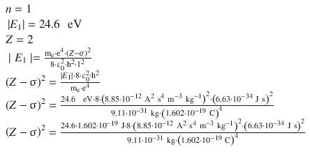
11.1. NaCl crystallises in the lattice type sodium chloride ( M = 1.747565) with r 0 = 2.82 Å and ρ = 0.321 Å. Calculate the lattice energy of NaCl.
The lattice energy of an ionic crystal can be calculated by the following expression:
We thus require the following parameters:
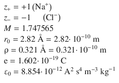
This yields:
The lattice energy of sodium chloride is −763 kJ mol −1 .
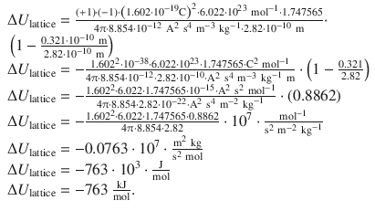
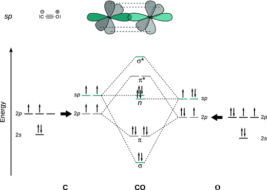
11.2. Discuss the bonding of carbon monoxide (CO) using the valence bond theory without and with hybridised atomic orbitals as well as the molecular orbital theory. Compare the bond order derived by the three approaches.
(a) VB theory:
![]()
Several resonance structure can be drawn for CO:
1. (i)
2. (ii)
3. (iii)
For (i) and (iii), the octet rule is nor satisfied for carbon, making the triple bond structure more favourable.
Experimentally, CO is found to possess a small dipole moment of 0.1 D; this suggests that structures with formal charges are less populated.
Overall, one could conclude for a bond order that is between a double and a triple bond.
(b) Hybrid orbitals:
The CO bonding can be explained by sp hybridisation which suggests two lone pairs ( n ) and predicts a bond order of:
![]() . (Note that the MO scheme above does not show the first shell electrons.)
. (Note that the MO scheme above does not show the first shell electrons.)
The overlap of one sp orbital of C and O each establishes a σ bond; the overlap of p y and p z orbitals of C and O established two π bonds: this suggests a C—O triple bond. One sp orbital on C and O each is occupied by a lone pair.
(c) MO theory:
Bond order:
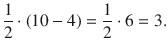
11.3. Determine for each of the species S − , Zn 2+ , Cl − and Cu + whether they are diamagnetic or paramagnetic.
S −
17 electrons
![]()
The ground state of S is [Ne] 3 s 2 3 p 4 . The extra electron is added to the 3p orbitals and renders a species with one unpaired electron. Therefore, S − is paramagnetic.
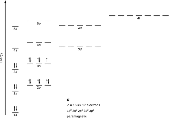
Zn 2+
28 electrons
![]()
The ground state of Zn is [Ar] 3 d 10 4 s 2 . In Zn 2+ , two electrons are removed from the 3 d orbital, rendering a species with two unpaired electrons, hence Zn 2+ is paramagnetic.
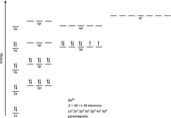
Cl −
18 electrons
![]()
With the ground state of Cl being [Ne] 3 s 2 3 p 5 , the extra electron completes the octet of the third shell and Cl − attains noble gas configuration. There are no unpaired electrons, hence Cl − is diamagnetic.
Cu +
28 electrons
![]()
The ground state configuration for Cu is [Ar] 3 d 10 4 s 1 . In Cu + , the 4 s 1 electron is removed and the outer shell is now 3 d 10 , which has no unpaired electrons. Therefore Cu + is diamagnetic.
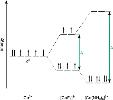
11.4. Using an appropriate molecular orbital scheme, explain why [Co(NH 3 ) 6 ] 3+ is a diamagnetic low-spin complex, whereas [CoF 6 ] 3− is a paramagnetic high-spin complex.
The ground state electron configuration of Co is 1 s 2 2 s 2 2 p 6 3 s 2 3 p 6 3 d 7 4 s 2 . In both complexes, cobalt takes the oxidation state +3, and has thus lost three electrons: two from the 4 s and one from the 3 d orbitals. The resulting electron configuration is thus 3 d 6 .
[Co(NH 3 ) 6 ] 3+
According to the spectrochemical series, NH 3 is a ligand that elicits a strong field, hence the crystal field splitting Δ is large. The six electrons are filled into the three low lying d orbitals which results in a low-spin, diamagnetic species.
[CoF 6 ] 3−
According to the spectrochemical series, F - is a ligand that elicits a weak field, hence the crystal field splitting Δ is small. The first three electrons populate the low lying d orbitals, then the fourth and fifth electrons occupy the high-lying d orbitals. The sixth electron pairs up with an electron in the low-lying d orbitals. This results in a high-spin, paramagnetic species.
Chapter 12
12.1. The dipole moment of HF is 1.92 D.
1. (a)
✵ The attractive arrangement of the two permanent HF dipoles in the plane along the x -axis can be illustrated as:
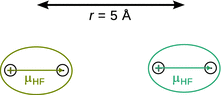
✵ The potential energy for this orientation is given by
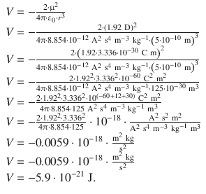
1. (b)
✵ For 1 mol HF:
1. (c)
Average thermal energy of bulk matter:
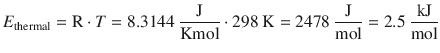
The dipole—dipole interaction is stronger than the thermal motion and can be sustained at 25 °C.
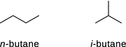
12.2. Explain why the boiling point of the two isomers of butane, n -butane and i -butane, are different. Which isomer has the higher boiling point?
Being isomers, n -butane and i -butane (2-methylpropane) have the same chemical formula C 4 H 10 . The isomers differ in their structures; whereas n -butane is an unbranched alkane, i -butane is branched:
Stronger inter-molecular forces result in a higher boiling point, as they must be overcome to free molecules into the gas phase. Of the different inter-molecular forces, only London dispersion forces apply to butane as both isoforms are alkanes and neutral molecules (no charge). They possess no hetero-atoms (i.e. C and H only) and thus no permanent dipole.
The longer, unbranched n -butane molecule has a larger surface area which provides more possibilities to anneal to neighbouring molecules and thus exert/experience dispersion forces. With i -butane being more compact, there are less dispersion forces between neighbouring molecules.
n -butane therefore has the higher boiling point.
This conclusion agrees with the literature values for the boiling points of n - and i -butane:
Table B.10
Comparison of the boiling points of butane isomers
Boiling point |
|
n -butane |
0 °C |
i -butane |
−11 °C |
Therefore, T b ( n -butane) > T b ( i -butane).
12.3. In which of the following substances are molecules held together by hydrogen bonds? Draw the hydrogen bonds where applicable.
1. (a)
✵ Since this does not contain hydrogen, there are no hydrogen bonds possible in XeF 4 .
1. (b)
✵ Whereas hydrogen is bonded covalently to carbon, the latter is not very electronegative and possesses no lone pairs. CH 4 is a non-polar molecule and does not exhibit hydrogen bonds.
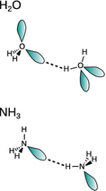
1. (c)
✵ There is a considerable electronegativity difference between oxygen and hydrogen and the lone pairs of oxygen engage in intra-molecular hydrogen bonds.
1. (d)
✵ This is not a covalent molecule, but rather an ionic structure consisting of Na + and H - (hydride) ions. There are no hydrogen bonds possible.
1. (e)
✵ Boron is less electronegative than hydrogen, hence hydrogen is not experiencing sufficiently positive partial charge; there are not hydrogen bonds.
1. (f)
✵ Compared to hydrogen, nitrogen is considerably more electronegative (polar N—H bond) and also possesses a lone pair which can engage in hydrogen bonding.
1. (g)
✵ There is no hydrogen bonding; iodine is not sufficiently electronegative to generate a polar H—I bond.
12.4. What is the relationship of the interaction energy between two particles due to Coulomb forces and dispersion forces with the distance? Compare the falloff of these energies with distance by calculating their ratio for the distances 1, 2, 3, 4 and 5 Å. Based on these results, assess the implications for ideal/non-ideal behaviour of solutions.
The Coulomb force depends on the charges on the two particles as well as their distance as per

and is thus indirect proportional to the distance: ![]() .
.
In contrast, the London dispersion force for a mixture of two particles A and B is given by
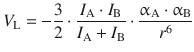
and therefore indirect proportional to the sixth power of the distance: ![]() .
.
Table B.11
Comparison of Coulomb and dispersion force falloff with distance
|
Distance |
Coulomb falloff |
Dispersion falloff |
Ratio |
r (Å) |
r −1 (Å −1 ) |
r −6 (Å −6 ) |
Coulomb:Dispersion falloff |
1 |
1.00000 |
1.00000 |
1 |
2 |
0.25000 |
0.01563 |
16 |
3 |
0.11111 |
0.00137 |
81 |
4 |
0.06250 |
0.00024 |
256 |
5 |
0.04000 |
0.00006 |
625 |
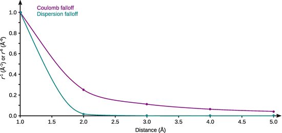
This (simplified) analysis shows that Coulomb forces between charged particles fall off much slower with separation distance than the weak dispersion forces. At a separation distance of 5 Å, Coulomb forces are several 100 times more pronounced than the weak dispersion forces. Therefore, even in dilute solutions, where the average separation distance of particles is large, Coulomb forces are major contributors.
For a solution to be ideal it is required that the interactions of solvent—solvent, solvent—solute, and solute—solute molecules are identical. This is clearly not the case when electrolytes are present, hence ionic solutions typically show non-ideal behaviour (which has implications for colligative properties; concentrations need to be replaced by activities, etc).
Chapter 13
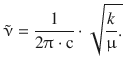
13.1. The infrared spectrum of carbon monoxide shows a vibration (v = 0 → v = 1) band at 2176 cm −1 . What is the force constant of the C—O bond, assuming the molecule behaves as a harmonic oscillator?
The frequency of the harmonic oscillator is given by ![]() , and the wavenumber is related to the frequency as per
, and the wavenumber is related to the frequency as per ![]() . Therefore:
. Therefore:
The reduced mass μ needs to be calculated using particular isotopes ( 12 C and 16 O), yielding
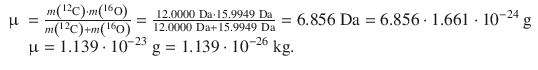
The force constant can now be calculated as follows:
13.2. Determine the ratio of populations of the vibrational levels v = 1 and v = 0 for carbon monoxide at 300 K and 1000 K. The wavenumber for the transition from v = 0 to v = 1 is 2176 cm −1 .
The population ratio is given by the equation based on the Boltzmann statistics:
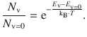
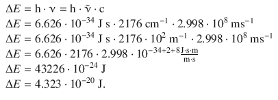
The difference ( E v − E v=0 ) is the energy difference between the two vibrational levels and can be accessed via the wavenumber observed for this transition:
For T = 300 K, the population ratio is then:
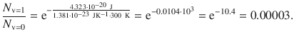
For T = 1000 K, the population ratio is:
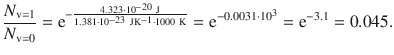
Whereas at 300 K, the first excited vibrational mode is virtually not populated, at 1000 K, about 4.5% of the CO molecules populate the mode v = 1.
13.3. Which spectroscopic symbol denotes the ground state of Li? What is the symbol of the lowest excited state? What feature can be deduced for the spectral line in the optical spectrum for this transition?
Li ground state:
Electronic configuration |
1 s 2 2 s 1 |
Quantum numbers of the valence electron |
n = 2, l = 0, m s = 1 / 2 , j = 0 + 1 / 2 = 1 / 2 |
Total spin |
S = |Σ s i | = |+ 1 / 2 — 1 / 2 + 1 / 2 | = 1 / 2 |
Spin multiplicity |
M = 2· S + 1 = 2· 1 / 2 + 1 = 2 |
Spectroscopic symbol |
2 S 1/2 |
Li first excited state:
Electronic configuration |
1 s 2 2 p 1 |
Quantum numbers of the valence electron |
n = 2, l = 1, m s = 1 / 2 , j = 1 + 1 / 2 = 3 / 2 n = 2, l = 1, m s = − 1 / 2 , j = 1 - 1 / 2 = 1 / 2 |
Total spin |
S = |Σ s i | = |+ 1 / 2 — 1 / 2 — 1 / 2 | = 1 / 2 |
Spin multiplicity |
M = 2· S + 1 = 2· 1 / 2 + 1 = 2 |
Spectroscopic symbol |
2 P 3/2 and 2 P 1/2 |
The transition from the ground state to the first excited state can be from 2 S 1/2 to either 2 P 3/2 or 2 P 1/2 . The spectral line therefore appears as a doublet with the individual lines having slightly differing energies.
13.4. In the free electron molecular orbital method, the π electrons in an alkene with conjugated double bonds are assumed to be freely moving within extent of the conjugation system. The conjugation system can be treated as a one-dimensional box.
1. (a)
2. (b)

1. (a)
1. (b)
✵ The energy of a particle in the one-dimensional box is given by
✵ This yields for the energy difference of the transition:
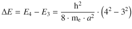
✵ The wavelength is obtained as per:
✵ Therefore:
13.5. How many lines/clusters are to be expected in the 1 H-NMR spectra of (a) benzene, (b) toluene, (c) o -xylene, (d) p -xylene, (e) m -xylene?
Protons |
Lines/clusters |
δ (ppm) |
|
(a) benzene |
6 aromatic H |
Singlet |
7.33 |
(b) toluene |
2+2+1 aromatic H 3 methyl H |
Multiplet Singlet |
7.00—7.38 2.34 |
(c) o -xylene |
2+2 aromatic H 6 methyl H |
Multiplet Singlet |
7.22—7.28 2.40 |
(d) p -xylene |
4 aromatic H 6 methyl H |
Singlet Singlet |
7.24 2.48 |
(e) m -xylene |
1 aromatic H 2+1 aromatic H 6 methyl H |
Doublet of doublet Multiplet Singlet |
7.28—7.31 7.11—7.14 2.47 |
13.6. Predict the number of hyperfine lines in the proton coupling observed in the ESR spectrum of the benzene anion radical C 6 H 6 − .
The six protons in the benzene anion are chemically equivalent ( N = 6); the nuclear spin of the proton is I = 1 / 2 . Therefore:
The benzene anion radical shows seven lines in the proton hyperfine coupling.
13.7. Determine the Raman and infrared activity of one symmetric and two different anti-symmetric vibrational modes of the square planar molecule XeF 4 .
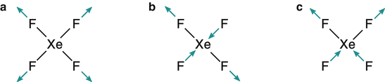
The symmetric stretching mode (a) does not lead to a change in the dipole momentum, but a change in the distribution electrons, i.e. polarisability. This mode is thus IR inactive and Raman active.
The anti-symmetric stretching mode (b) does not lead to a change in the dipole momentum but to a change in the electron distribution (polarisability). This mode is therefore IR inactive and Raman active.
The anti-symmetric stretching mode in (c) does indeed lead to a change in the dipole momentum as the individual dipole momentum changes by bond stretching on opposite sides do no longer cancel. The overall electron distribution does not change, since the compression on one side of the molecule is compensated for by an expansion on the other side; the polarisability does not change. Therefore, this mode is Raman inactive, but IR active.