Physical Chemistry Essentials - Hofmann A. 2018
Thermodynamics
2.3 Properties of Real Systems
In the previous sections, we have focused on single component systems whose composition does not change. This is clearly a limitation, since many real systems (as opposed to ideal systems) consist of multiple components and we thus need to consider varying compositions.
When considering the free energy of real systems it proves useful to introduce three new properties:
✵ chemical potential
✵ fugacity
✵ activity
2.3.1 Chemical Potential
In the previous section, we derived a relationship that enables calculation of the free energy of an ideal gas at any given pressure:
![]()
(2.66)
If we consider 1 mol of the ideal gas, this becomes:
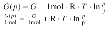
The reference to the molar amount of 1 mol is indicated by the subscript ’m’:
![]()
(2.67)
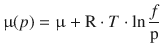
thereby introducing G m as the molar Gibbs free energy and thus the chemical potential μ:
![]()
(2.67)
The term ’potential’ is chosen based on the idea that for mechanical systems, the lowest potential energy is the most stable state. Similarly, the state of a system with the lowest chemical potential constitutes the most stable state, since for all spontaneous processes
![]()
From the point of view of varying compositions, the change of the chemical potential μ equals the change of the free energy of the system, if a molar amount of n = 1 mol more substance is added.
The chemical potential μ is thus the molar free energy of a substance, and therefore an intensive property; its value is independent of the amount, since it has been normalised against 1 mol substance.
2.3.2 Open Systems and Changes of Composition
If we are dealing with chemical and biological systems comprising of multiple components, the composition will likely change. Sometimes, substances may even leave the system under observation; such systems are called open systems. We thus need to consider changes in the molar amount of substance in the system.
So far, we have assumed that the state of a system can be expressed as a function of two variables, say T and p. However, if the composition changes, the state also depends on the molar amount of each substance:
![]()
To evaluate the change of the free energy of the system, we therefore need to consider the change in all properties, including the amount of each component. This can be expressed as the differential of the Gibbs free energy with respect to each of the variable parameters (p, T, n i ):
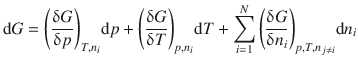
(2.68)
Form earlier considerations in Sect. 2.2.7, we know how the Gibbs free energy varies with pressure and temperature:
![]()
(2.64)
And we also know that the chemical potential m is the change of the free energy of a substance when changing its molar amount (’adding 1 mol’):
(2.67)
If we substitute Eqs. 2.64 and 2.67 into Eq. 2.68, we obtain the fundamental equation of thermodynamics:
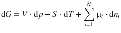
(2.69)
In chemical and biological systems (e.g. electrochemical or biological cells), T and p often remain constant, but the composition changes. For example, the intra- and extracellular metal ion concentration in cells is markedly different (Table 2.6):
Table 2.6
Extra- and intra-cellular concentrations of biologically important metals
Extra-cellular |
c(Na+) = 140 mM |
c(K+) = 4 mM |
c(Ca2+) = 9 mM |
Intra-cellular |
c(Na+) = 12 mM |
c(K+) = 139 mM |
c(Ca2+) < 0.2 mM |
Muscle cells expend energy to transport calcium ions to the outside of the cells. The calcium ions that flow into the muscle cells promote the cross-bridging between two fibre proteins (actin and myosin) which ultimately causes contraction. It is thus the change of chemical composition that drives this biological reaction.
2.3.3 Fugacity: A Pressure Substitute for Non-ideal Gases
When we derived the chemical potential in Sect. 2.3.1, we have been considering a system that contained an ideal gas:
![]()
(2.67)
Real gases, i.e. such that behave in a non-ideal fashion, don’t fulfil some or all of the criteria we have requested for an ideal gas. The ideal gas equation poses that the product (p·V) remains constant at constant temperature; the value of (p·V) should thus be independent of the pressure. However, experimental observation for real gases shows that this is not the case. To account for these deviations, The ideal gas equation may be extended by additional terms containing virial coefficients (B, C, D, …):
![]()
(2.70)
These deviations include the observation that the volume of a gas may change under certain circumstances, even if pressure and temperature remain constant, e.g. when the gas condenses to a liquid. Since the existence of a condensed phase is not possible without intermolecular interactions, it becomes clear that a central requirement for an ideal gas is being violated.
In order to adjust the chemical potential such that one can also accommodate non-ideal behaviour, a new property called fugacity f is defined. The fugacity constitutes an adjusted pressure and is related to the pressure by a scalar factor called the fugacity coefficient ϕ:
![]()
(2.71)
Fugacity is thus measured in units of pressure: [f] = 1 Pa.
The fugacity of a gas expresses its tendency to escape (being fugitive). This is intimately connected with how compressible the real gas is, compared to the ideal gas.
It is common to use an implicit definition of the fugacity: it is the property that replaces the pressure p in the definition of the chemical potential, thus ensuring that the following equation remains valid even in the case of non-ideal behaviour:
(2.72)
The difference between pressure and fugacity, and thus the extend of deviation from ideal gas behaviour, is illustrated in Table 2.7 for nitrogen at various pressures.
Table 2.7
Fugacities and fugacity coefficients for N2 at T— = 273.15 K
|
p (bar) |
ϕ |
f (bar) |
50 |
0.98 |
49 |
100 |
0.97 |
97 |
200 |
0.97 |
194 |
400 |
1.06 |
424 |
600 |
1.22 |
732 |
800 |
1.47 |
1176 |
1000 |
1.81 |
1810 |
2.3.4 Solutions
When we consider solutions or mixtures, characteristic properties for the system under observation are the concentrations of individual components in the system. In addition to the well-known molar concentration that defines the molar amount of a substance in a particular volume of solution
![]()
(2.73)
it may be more convenient to use further measures of concentration, depending on the system under study (for a summary see Sect. 4.3.2). Here, we want to focus in particular on
✵ the mole fraction: x i
✵ the partial molar volume: v i
Mole Fraction
The mole fraction is defined as the molar amount of an individual component divided by the total molar amount in a system:
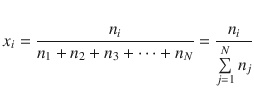
(2.74)
In the above notation, the index i denotes an individual compound from the set (1, 2, 3, …, N). The running index on the sum in the denominator of the quotient thus needs to be a different character (here j) to indicate that it is independent of i.
For gas mixtures, the mole fraction can be calculated based on the partial pressure of the individual components:
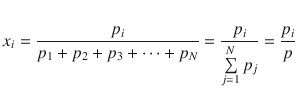
(2.75)
The mole fraction is a frequently used measure of concentration in gas, liquid and solid phase systems.
Partial Molar Volume
The partial molar volume of a particular substance is defined as the change in volume of a mixture, when 1 mol of the particular substance is added. One can thus express the partial molar volume as the change of the volume of the entire system when changing the molar amount of the particular substance in the system:
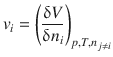
(2.76)
In the above expression, the index i denotes an individual substance, and the subscripts to the right of the differential inform us that not only the pressure and temperature need to remain constant during the addition of further amounts of the i-th substance, but also the amounts of all other substances in the system (denoted by the index j which has to be different from i) need to remain constant.
The partial molar volume is a function of the composition of the mixture to which it is added, i.e. the partial molar volume is not a constant for a given substance!
Notably, gases and liquids behave differently, due to the existence of inter-molecular interactions: If two different ideal gases are combined, the total volume is the sum of the individual volumes of each gas. However, if two different liquids are combined, the total volume is not the sum of each, due to the interactions between the liquids.
Example
If 1 mol of water is added to a very large volume of water, the change in volume is 18 ml.
However, if 1 mol of water is added to a very large volume of ethanol (so large that each water molecule is surrounded by ethanol molecules) then the increase is just 14 ml.
The partial molar volume of water in pure water is v(H2O, H2O) = 18 ml mol−1, the partial molar volume of water in pure ethanol is v(H2O, EtOH) = 14 ml mol−1.
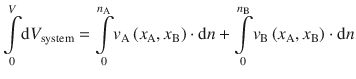
Once determined, the partial molar volume can be used to determine the change in volume of system composed of two components (A and B), when a known amount of A is added to a solution:
![]()
Integration of this equation yields the total volume of a system with known composition:
All integrals in above equation are of the type 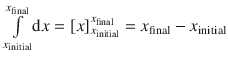 , so the equation resolves to:
![]()
2.3.5 The Gibbs-Duhem Equation
In the previous section, by means of describing concentrations, we have expressed the volume of a multi-component system as function of the molar amounts of the individual components.
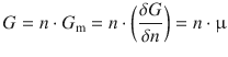
In the same way, other properties such as e.g. the Gibbs free energy of a mixture can be expressed in terms of the molar composition:
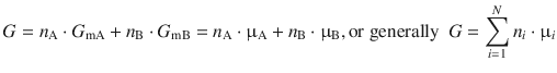
(2.77)
The above expression allows calculation of the Gibbs free energy (extensive!) based on knowledge of the molar amounts of the individual components as well as their chemical potentials (intensive!).
The molar functions we have introduced so far include:
✵ molar Gibbs free energy = chemical potential (a partial molar function when it refers to an individual component)
✵ partial molar volume
✵ mole fraction (a partial molar function as it relates to an individual component)
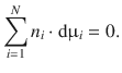
If the partial molar function (e.g. the chemical potential or the partial molar volume) of one component of a mixture changes, it must be balanced by the opposing change in the partial molar functions of the other.
For example, when adding an additional volume of liquid to a solution, the partial molar volume of that substance increases, while the partial molar volumina of all other components decrease:
Applying the same considerations to the chemical potential, one obtains the Gibbs-Duhem equation: