5 Steps to a 5: AP Microeconomics 2017 (2016)
STEP 4
Review the Knowledge You Need to Score High
CHAPTER 10
Factor Markets
IN THIS CHAPTER
Summary: We have invested significant time reviewing the forces of supply and demand in the competitive market for goods and services. In addition, we have investigated the theory behind production and cost, but have not brought market forces to bear on those input, or factor, markets. We begin with the demand for inputs in a perfectly competitive input market, and then move to the supply of inputs and construct a model of wage and employment. We tweak the competitive model by allowing for some monopoly hiring behavior. How is the wage of college professors determined? Can we predict whether employment of steel workers is going to grow or decline? A study of input markets sheds some light on many important microeconomic issues that have critical macroeconomic implications.

Key Ideas
![]() Factor Demand
Factor Demand
![]() Least-Cost Hiring of Inputs
Least-Cost Hiring of Inputs
![]() Factor Supply
Factor Supply
![]() Equilibrium in Competitive Factor Markets
Equilibrium in Competitive Factor Markets
![]() Non-Competitive Factor Markets
Non-Competitive Factor Markets
10.1 Factor Demand
Main Topics: Competitive Factor Markets, Marginal Revenue Product, Profit-Maximizing Resource Employment, MRP L as Demand for Labor, Derived Demand, Determinants of Resource Demand
The theory of factor (or resource, or input) demand is applicable to any factor of production, but it is more intuitive if we focus on labor, the production input with which we are all most comfortable. Because we are most familiar with it, most examples below address labor, but later in the chapter we will also look at the market for capital.
Competitive Factor Markets
To best see the theory of factor demand, we assume the simplest market structure. First, we’ll assume that the firms are price takers in the product (output) market. Second, we’ll assume that they are price takers in the factor (input) market. This means that they cannot impact either the price of their product or the price they must pay to employ more of an input. In a competitive labor market, they can employ as much labor as they wish at the going market-determined wage.
Marginal Revenue Product
Here’s a difficult question for any employee to ask: What am I worth to my employer? Sure, I’m a snazzy dresser; I can tell a humorous joke, and my personal hygiene is top-notch. However, the bottom line to my employer is probably more important than these civilities. To build a model of factor demand, economists assert that the demand for a unit of labor is a function of two things important to employers. First, employers are very interested in the marginal productivity of the next unit of labor. If the next worker is going to greatly contribute to the firm’s total production, he is likely to be a good hire for the firm. Second, the firm must then receive good value for the production. The value of this production to the firm is the additional, or marginal, revenue that it brings to the firm. Combining the necessary components of marginal productivity of labor and marginal revenue provides marginal revenue product of labor (MRP L ), a measure of what the next unit of a resource, such as labor, brings to the firm. With the assumption of a perfectly competitive output market, the marginal revenue is simply the price of the product.

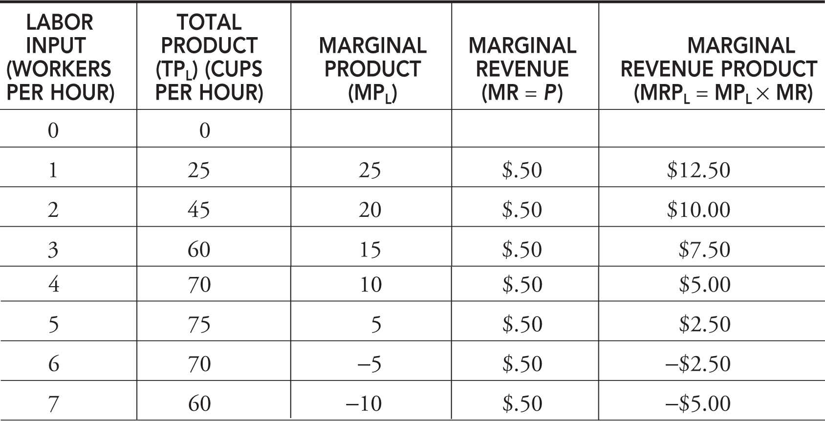
In our examples, we change the resource (labor) by a quantity of one. Table 10.1 revises the hourly production function for Molly’s lemonade stand. Recall that in the short run she hires additional units of labor to a fixed level of capital. The competitive price of a cup of lemonade is 50 cents.
Table 10.1
Profit-Maximizing Resource Employment
Yet again, we are faced with a decision that must be based upon marginal benefits and marginal costs. Our decision rule is, and has always been:

• If MB > MC, do more of it.
• If MB < MC, do less of it.
• If MB = MC, stop here.
In the case of resource hiring, the marginal benefit is MRP L . The marginal cost of resource hiring is marginal resource cost (MRC ), a measure of how much cost the firm incurs from using an additional unit of an input. When the firm is hiring labor in a competitive labor market, MRC is equal to the wage (w ).

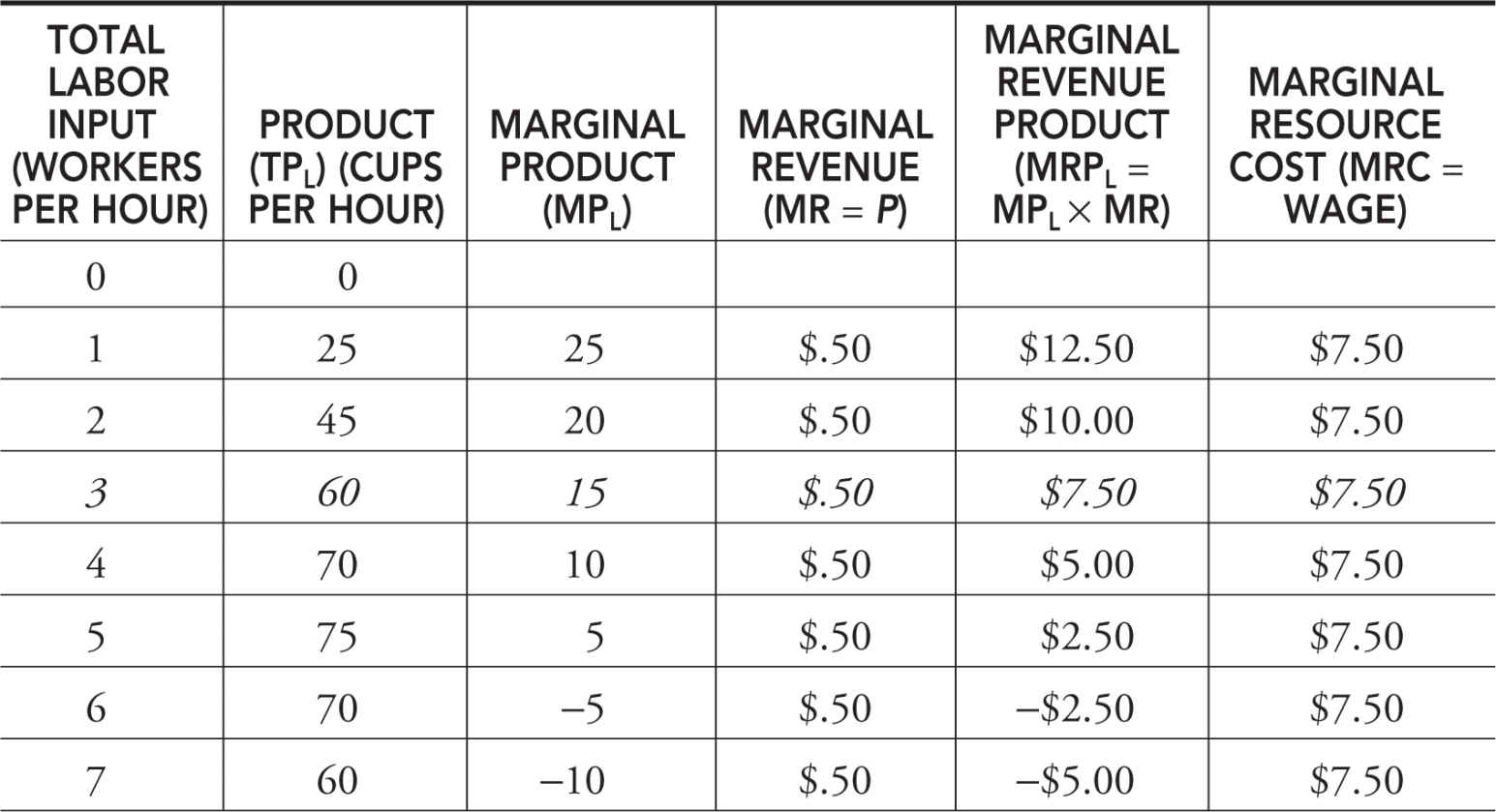
With this measure of marginal cost, the profit-maximizing employer of labor would hire to the point where MRPL = MRC = Wage. Table 10.2 adds a competitive $7.50 hourly wage to Molly’s table of lemonade production. At this wage, Molly should employ three hourly workers to her fixed capital.
Table 10.2
MRPL as Demand for Labor
If the hourly wage were to rise to $10, Molly would reduce her employment to two workers per hour. If the wage decreases to $5 per hour, she would employ four workers. All else equal, as the price of labor increases, the employment falls and as the price of labor decreases, employment rises. This is the law of demand again! Figure 10.1 illustrates the MRPL and Molly’s hiring at three wages.
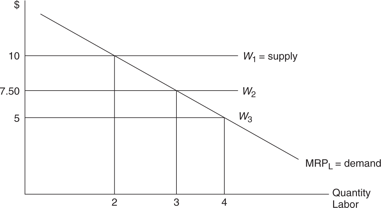
Figure 10.1
Molly’s demand for labor is actually represented by the MRPL . It is downward sloping, like any demand curve would be, because of the diminishing marginal productivity of labor in the short run. To move from Molly’s demand for labor to the overall market demand for labor, we simply sum up all of the individual firms’ MRPL curves: Market DL = ΣMRPL .
Market Wage as Supply of Labor
Under the assumptions of a perfectly competitive labor market, the supply of labor to the individual firm is perfectly elastic and equal to the wage. This means that the firm can employ all of the workers it desires at the going market wage.
• In competitive markets, MRPL is the firm’s labor demand curve.
• In competitive markets, wage is the firm’s labor supply curve.
Derived Demand
Economists say that the demand for an input like labor is derived from the demand for the goods produced by the input. If the weather is hot and demand for lemonade rises, local economists might predict a stronger demand for production resources like lemonade workers, lemons, and sugar. An increase in the demand for a resource means that at any wage, the firm wishes to employ more of that resource. If the demand for lemonade increases and the price rises to $1 per cup, the MRPL increases at all quantities of labor. This is seen in Figure 10.2 .
• You are very likely to see the topic of derived demand on the AP exam. To avoid losing points on the free-response question, you must make the connection between the price of the product rising and the increased demand for the labor.
• ↑D for product, ↑price of product, ↑MRPL , ↑hiring of labor at the current wage.
Determinants of Resource Demand
The demand for the goods themselves is an important determinant of resource demand, but not the only determinant.
“Keep answers crisp, graphs labeled, and you are on your way to a 5.”
—Navin, AP Student
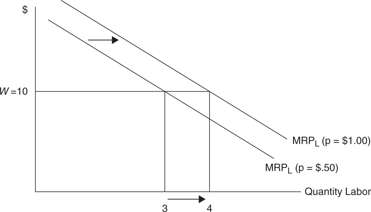
Figure 10.2
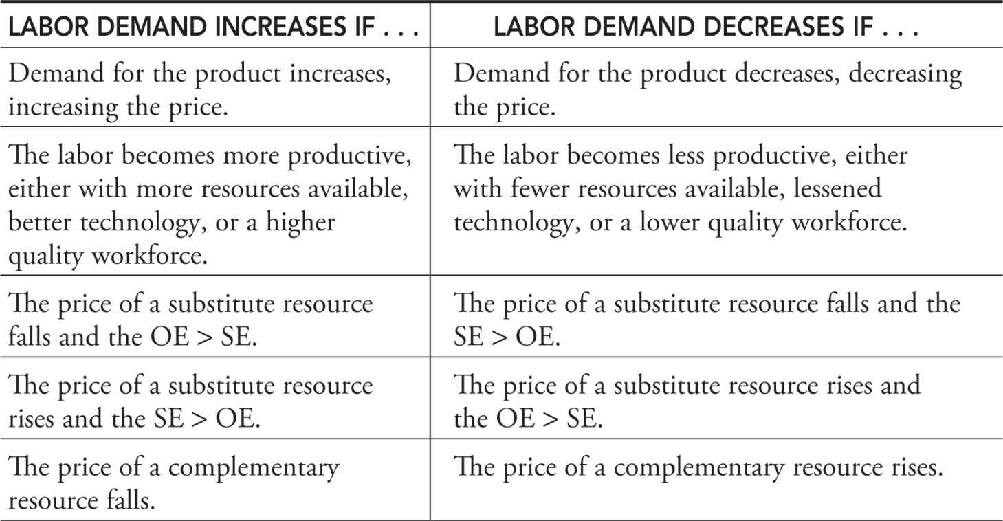
• Product demand . An increase in the demand for textiles—towels, for example—results in an increased price of those goods. The higher price increases the marginal revenue product of resources used in the production of textiles (e.g., textile workers), and this shifts the demand for those resources to the right. Of course, this works in the opposite direction and is probably a more accurate story of what has happened to textile workers in the United States.
• Productivity (output per resource unit ). If the productivity of the resource increases, the firm has a profit motive to take advantage of that heightened productivity and the demand for the resource should increase. Productivity of a resource is affected by a few different factors:
1. Quantity of other resources . Give workers more equipment to help production and labor’s productivity can be increased. If Molly were to provide her workers with a larger workspace or more manual juicers or pitchers or stirring spoons or measuring cups, they might achieve increased output per worker.
2. Technical progress . Better technology with which to work can increase labor’s productivity. Rather than using manual lemon squeezers, Molly invests in electric squeezers that allow for a given number of employees to produce more lemonade every hour.
3. Quality of variable resources . Fertile farmland in the Midwest is a huge productivity advantage over the same acreage of farmland in Nevada. A more educated and trained workforce is an improvement in the quality of the labor and therefore provides more productivity. Maybe Molly employs only those who have completed daylong training at the local community college.
• Prices of other resources . Employers hire several different resources, so the demand for one (labor) often depends upon the prices of the others.
1. Substitute resources . If the price of a substitute resource—machinery, for example—falls, it has two competing effects on the demand for labor.
a. Substitution effect (SE). Because machinery is now relatively less expensive, the firm uses more machinery and decreases demand for labor. For Molly, a lower price of electric lemon squeezers would put pressure on her to decrease the demand for labor.
b. Output effect (OE). Lower machine prices lower production costs (a downward shift in MC), which increases output for the firm and prompts an increased demand for labor. With the lower marginal cost of producing lemonade, Molly sees that she can actually produce more and would therefore need more labor.
c. The net effect of a lower price of capital depends upon the magnitude of each effect. If the SE > OE, demand for labor falls. If the OE > SE, the demand for labor increases.
2. Complementary resources . When labor and machine work together, a lower price of the machine makes it more affordable to purchase more machinery but also increases the demand for labor. Interstate trucking companies need trucks, fuel, and drivers. When the price of fuel increases, this can have a negative impact on the demand for drivers. For Molly’s firm, if the price of lemons falls, this more affordable complement to labor might increase the demand for labor.
Table 10.3 is a summary of the determinants of labor demand.
Table 10.3
10.2 Least-Cost Hiring of Multiple Inputs
Main Topic: The Least-Cost Hiring Rule
Finding the best way to cope with scarcity really excites economists. We found that consumers needed to find the best (utility maximizing) combination of two goods, given the prices and an income constraint. For producers, we would like to find the best (cost minimizing) combination of two inputs, given the prices and production constraint. To do this, we use the consumer’s decision as a model for the producer’s decision. The consumer’s utility maximizing rule said to find the combination of good X and good Y so that MUx /P x = MUy /P y while spending exactly his or her income and paying prices P x and P y .
Least-Cost Hiring Rule
For a producer, we can express the constraint in two equivalent ways. Remember the bridge between production and cost?
1. You must produce Q * units of output. Now find the least-cost ($TC) way of doing so.
2. You can only spend $TC. Now find the highest level of output (Q* ).
There is only one combination of two resources (we’ll use labor and capital) that satisfies either of these two constraints, and it is found by using this least-cost rule . The price of labor is P L and the price of capital (K ) is P K .
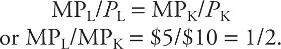
MPL /P L = MPK /P K , or equivalently, MPL /MPK = P L /P K
Example:
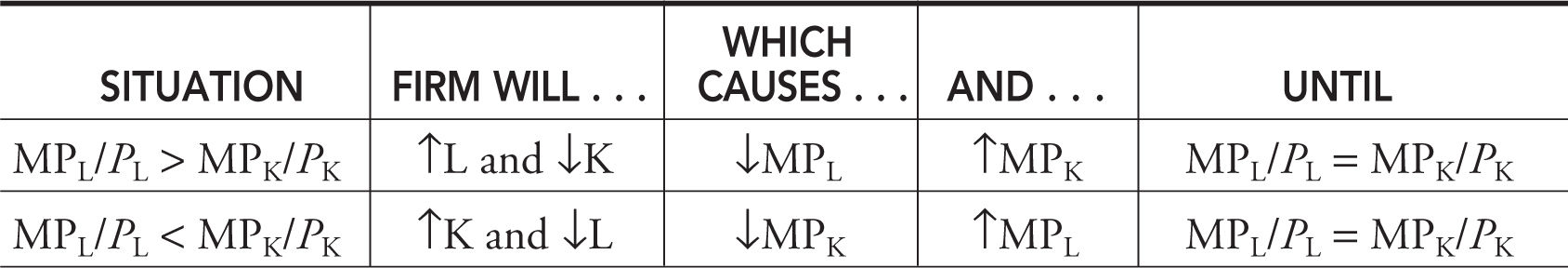
If each of the inputs is hired at $1 per unit and at the current amount of labor and capital you have employed, the MPL = 100 and the MPK = 10. Clearly, the least-cost rule is not satisfied:
100 units/$1 > 10 units/$1
If you could spend $1 more on labor, you would see output increase by 100 units. That extra $1 would come from spending $1 less on capital, which would decrease output by 10 units. So you spend the same amount of money but get 90 more units of output.
Great deal! In situations like this, where MPL /P L > MPK /P K , the firm is going to find it in its best interest to increase spending on L and decrease spending on K . The law of diminishing marginal returns predicts that as you increase L , MPL falls. And as you decrease K , MPK rises. The substitution of labor for capital ceases to be a great deal at the combination of L and K where the ratios of marginal product per dollar are equal again.
Example:
A producer of gadgets pays $5 for each hour of labor and $10 for each hour of capital employed. Table 10.4 describes the marginal products of each at various levels of employment. Told that you must produce Q = 360 gadgets, find the least-cost combination of labor and capital.
Table 10.4
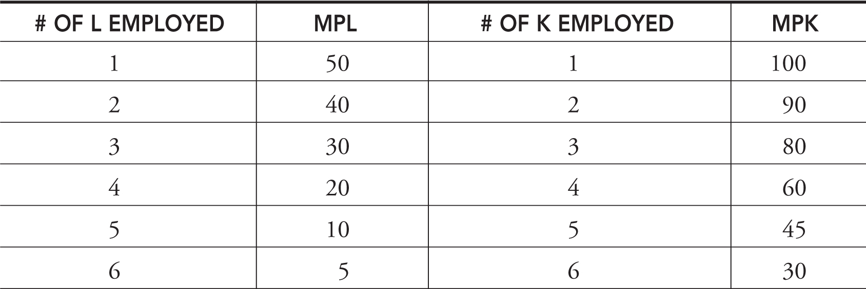
Find all of the combinations of L and K where our rule is satisfied:
There are three possibilities where the MPL is one-half the size of MPK :
• L = 1, K = 1. Total Product = 50 + 100 = 150
• L = 2, K = 3. Total Product = (50 + 40) + (100 + 90 + 80) = 360
• L = 3, K = 4. Total Product = (50 + 40 + 30) + (100 + 90 + 80 + 60) = 450
The best way to produce 360 gadgets is to hire two units of labor and three units of capital at a total cost of TC = $5 × 2 + $10 × 3 = $40. The same problem could have been modified to use a cost constraint rather than an output constraint.
Told that you can only spend $40, find the combination of labor and capital that maximizes production. Of course, the solution is again L = 2, K = 3, and output is 360 gadgets.
10.3 Factor Supply and Market Equilibrium
Main Topics: Supply of Labor, Wage and Employment Determination, What About Other Resources?
If you have ever had a job, you have been a small part of the labor supply curve. We quickly investigate labor supply and combine it with labor demand to complete a labor market. It is in this competitive market that wage and employment are determined.
Supply of Labor
Economic theory predicts that as the price of a good increases, suppliers of that good increase the quantity supplied. This is the law of supply . If the price of labor (wage) increases, more hours of labor should be supplied. For the most part, this is true, and the market labor supply curve slopes upward. If the hourly wage increased from $5 to $8, most people respond by working more hours, earning more income ($320 per 40-hour workweek), and consuming more goods.
Wage and Employment Determination
Assuming competitive output and input markets, the competitive wage is found at the intersection of labor demand and labor supply. Changing demand and supply influence this wage, and the equilibrium quantity of labor that accompanies it.
Example:
The aging population in the United States is giving a boost to the market for nurses. An increase in the demand for nurses increases both the wage and employment of nurses. This is seen in the Figure 10.3 .
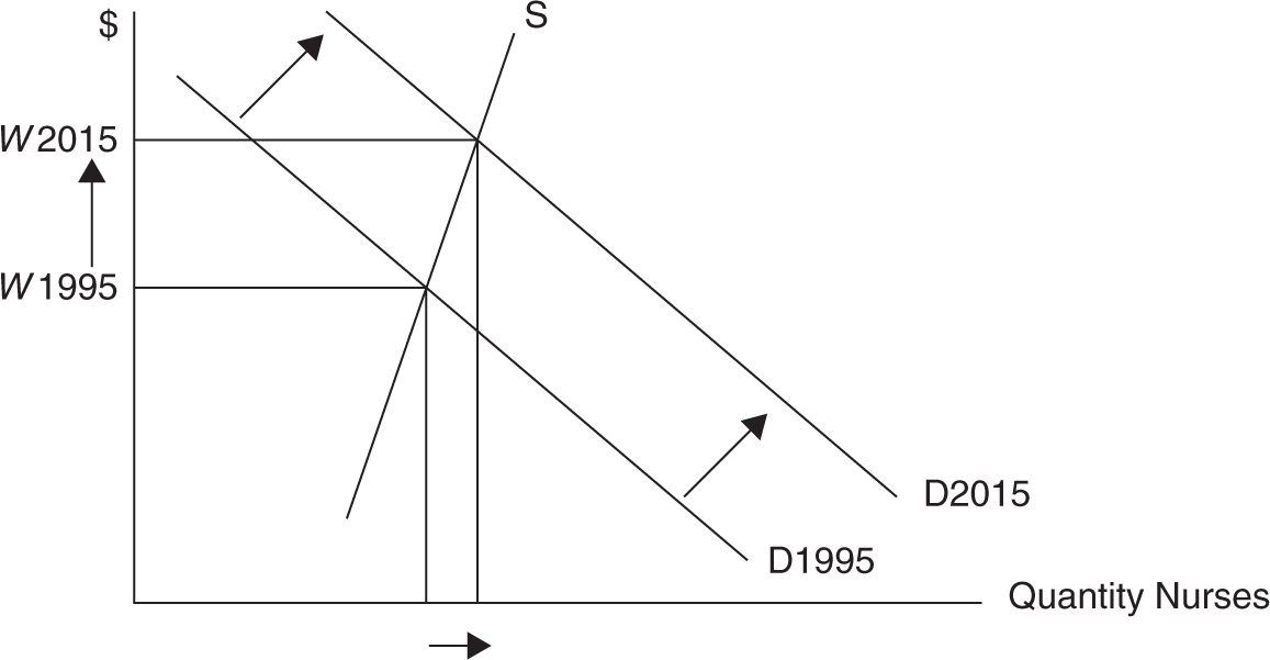
Figure 10.3
What About Other Resources?
Labor is the resource with which most people identify because we have all been, or expect to be, units of labor in a labor market. However, we can use the theory of resource demand to predict how the market for capital (or any other resource) would behave. For example, suppose that the market for capital is also perfectly competitive. If so, then each firm’s demand for capital is also derived from the marginal revenue product of capital (MRPK )
MPRK = P × MPK
And because the marginal product of capital diminishes, the demand for capital is downward sloping. In a competitive resource market, the firm can hire all of the capital it wants at the marginal factor cost equal to the rental rate of capital (r *).
Each firm hires the profit-maximizing quantity of capital (K *) at the point where the MRPK is equal to the rental rate (r *). We can see this hiring decision in Figure 10.4 .
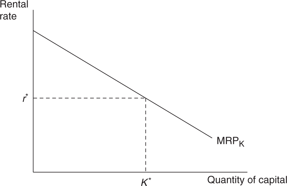
Figure 10.4
But where does this rental price of capital come from? With many firms hiring capital in this competitive market, the market demand for capital is downward sloping. The market supply curve for capital is upward sloping, and the market determines the competitive price of capital (r *). This is seen in Figure 10.5 .
Market forces, just as in the labor market, would cause the rental rate and quantity of capital to change. For example, if the demand for capital increases, perhaps because of a strong economy and positive corporate expectations, the equilibrium price and quantity of capital in the market would be expected to increase.
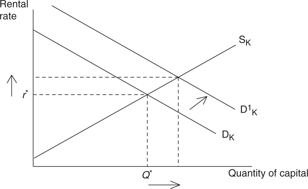
Figure 10.5
10.4 Imperfect Competition in Product and Factor Markets
Main Topics: Market Power in Product Markets, Market Power in Factor Markets
We saw in the previous chapter that perfectly competitive markets might not always exist. After all, the conditions for perfect competition are rather strict and not often observed in the “real world.” In the sections that follow, we assume that the firm has some market power, first in the product market and then in the factor (labor) market. To no surprise, the outcome of wage and employment differs from the competitive outcome described previously.
Market Power in Product Markets
Perhaps the most important result seen from a firm that has the ability to be a price setter is that the price exceeds marginal revenue. Because MR < P with market power, this has an impact on the marginal revenue product function.
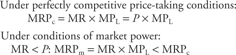
The result of a lower marginal revenue product function is that the optimal amount of employment falls at all wages. Figure 10.6 illustrates this. In other words, the monopolist hires lesser amounts of all resources, including labor. This should make sense if you recall that monopoly markets produce less output than the competitive market. If the market produces less output, it makes sense that the market would employ fewer resources.
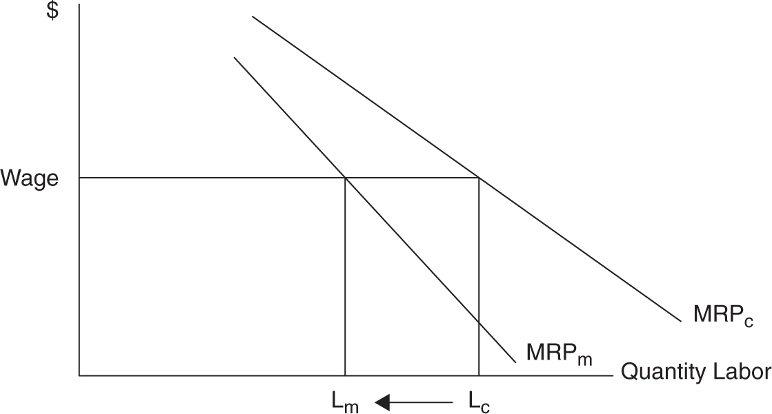
Figure 10.6
• Because MR < P , MRPm = MR × MPL < MRPc .
• A monopoly market employs fewer workers than the competitive market.
Market Power in Factor Markets
When a producer has extreme market power in the product market, we label them a price-setting monopolist, and the price of the product is set above marginal revenue. Let’s turn this situation around to the factor market. If an employer has extreme market power in the factor market, we label them a wage-setting monopsonist, and we observe the wage set below marginal factor cost.
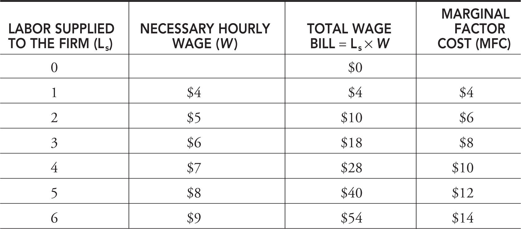
In a competitive labor market, the firm could employ all it wanted at the market-determined wage. The key difference between monopsony and a perfectly competitive labor market is that the employer must increase the wage to increase the quantity of labor that is supplied. In other words, the labor supply to the firm is upward sloping, not horizontal. Marginal factor cost is now greater than the wage. Table 10.5 illustrates how this happens.
Table 10.5
Example:
Molly’s lemonade conglomerate can employ more workers but must increase the wage to do so. However, not only does she have to increase the wage for additional workers but also to her current workers. This creates a situation where the MFC > W . See Figure 10.7 . Molly still chooses to employ where MRPL = MFC, but the wage is determined from the labor supply curve. Graphically the MFC curve lies above the labor supply curve, which means that labor is paid below their MRPL .
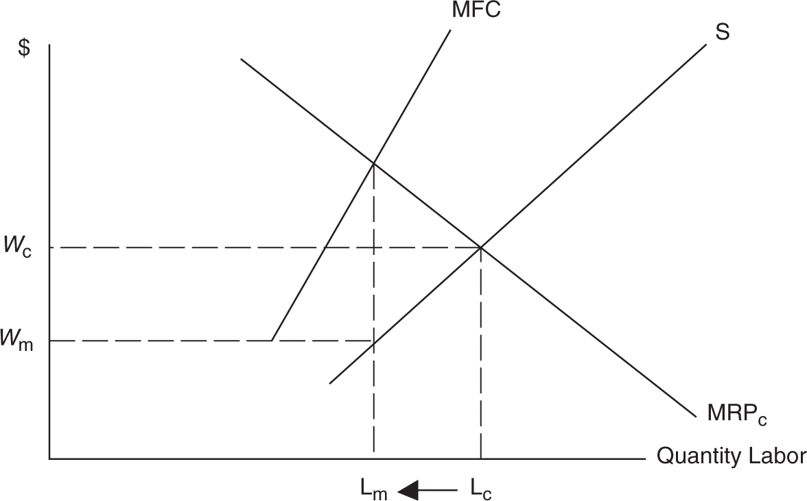
Figure 10.7
• Under monopsony, employers hire L m < L c .
• Monopsony firms pay W m < W c = MRPL .
Remember that MRPL measures the value of the last worker to the firm. The outcome that workers receive less than their value to the firm might be alarming. Does this happen? If you doubt that an employer can get away with such rampant exploitation, I give you a four-letter response: N-C-A-A. A big-time college star athlete might produce, over the course of a four-year career, millions of dollars in revenue to a university. Even if we include the value of four years of tuition, room, and board, the star athlete is compensated well below his or her marginal revenue product. Is it so crazy that many talented college athletes make an early jump to a professional league or in some cases skip college altogether?
![]() Review Questions
Review Questions
1 . Your aunt runs a small firm from her home making apple pies. She hires some friends to help her. Which of the following situations would most likely increase her demand for labor?
(A) The price of apple peelers/corers rises.
(B) Your aunt’s friends gossip all day, slowing their dough-making process.
(C) There is a sale on ovens.
(D) A new study reveals that apples increase your risk of cancer.
(E) The price of apples increases.
2 . The price of labor is $2, and the price of capital is $1. The marginal product of labor is 200, and the marginal product of capital is 50. What should the firm do?
(A) Increase capital and decrease labor so that the marginal product of capital falls and the marginal product of labor rises.
(B) Increase capital and decrease labor so that the marginal product of capital rises and the marginal product of labor falls.
(C) Decrease capital and increase labor so that the marginal product of capital rises and the marginal product of labor falls.
(D) Decrease capital and increase labor so that the marginal product of capital falls and the marginal product of labor rises.
(E) Increase both capital and labor until the ratio of marginal products per dollar is equal.
3 . A competitive labor market is currently in equilibrium. Which of the following most likely increases the market wage?
(A) More students graduate with the necessary skills for this labor market.
(B) Demand for the good produced by this labor is stronger.
(C) The price of a complementary resource increases.
(D) The Department of Labor removes the need for workers to pass an exam before they can work in this field.
(E) Over time, one large employer grows to act as a monopsonist.
Use Table 10.6 to respond to questions 4 and 5.
Table 10.6
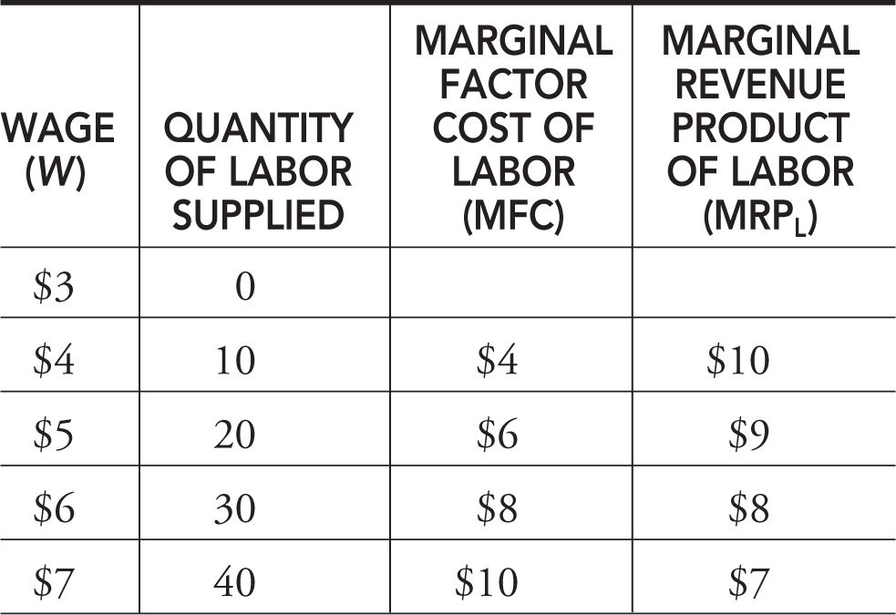
4 . If a firm is hiring labor in the perfectly competitive labor market, the wage and employment are
(A) $3 and zero.
(B) $4 and 10.
(C) $5 and 20.
(D) $6 and 30.
(E) $7 and 40.
5 . If a firm hires labor in a monopsony labor market, the wage and employment are
(A) $3 and zero.
(B) $8 and 30.
(C) $5 and 20.
(D) $6 and 30.
(E) $7 and 40.
![]() Answers and Explanations
Answers and Explanations
1 . C —Since ovens would be a less expensive complementary resource (with more ovens, they can bake more pies), your aunt needs more employees to go along with the extra ovens. Apple corers and peelers are complements, but even if you think they are substitutes, the impact on labor demand is uncertain because of the competing output and substitution effects.
2 . C —Do a quick ratio of marginal product per dollar. When you see that the MPL /P L > MPK /P K , you notice that the firm is getting more “bang for the buck” with labor. Immediately rule out any choice that says they hire less labor. The only way that MPL /P L falls to equal MPK /P K is to decrease the capital and increase the labor, causing the MPK to rise and the MPL to fall. The firm does this until the marginal products divided by the prices are equal.
3 . B —The equilibrium wage rises with stronger demand or lessened supply of labor. The stronger demand for the product increases the wage as the demand for labor increases. All other choices either increase the labor supply or decrease the demand, thus decreasing the wage. Emergence of monopsony decreases the wage below competitive levels.
4 . E —In a competitive labor market, equilibrium is where W = MRPL .
5 . D —In a monopsony labor market, equilibrium is where MFC = MRPL .
![]() Rapid Review
Rapid Review
Marginal revenue product (MRP): Measures the value of what the next unit of a resource (e.g., labor) brings to the firm. MRPL = MR × MPL . In a perfectly competitive product market, MRPL = P × MPL . In a monopoly product market, MR < P so MRPm < MRPc .
Marginal resource cost (MRC): Measures the cost the firm incurs from using an additional unit of an input. In a perfectly competitive labor market, MRC = Wage. In a monopsony labor market, the MRC > Wage.
Profit-maximizing resource employment: The firm hires the profit-maximizing amount of a resource at the point where MRP = MRC.
Demand for labor: Labor demand for the firm is the MRPL curve. The labor demand for the entire market DL = ΣMRPL of all firms.
Derived demand: Demand for a resource like labor is derived from the demand for the goods produced by the resource.
Determinants of labor demand: One of the external factors that influences labor demand. When these variables change, the entire demand curve shifts to the left or right.
Least-Cost Rule: The combination of labor and capital that minimizes total costs for a given production rate. Hire L and K so that MPL /P L = MPK /P K or MPL /MPK = P L /P K .
Monopsonist: A firm that has market power in the factor market, i.e., a wage setter.