5 Steps to a 5: AP Microeconomics 2017 (2016)

STEP 4

Review the Knowledge You Need to Score High

CHAPTER 7

Elasticity, Microeconomic Policy, and Consumer Theory

IN THIS CHAPTER

Summary: It is critical to remember that behind the faceless supply and demand curves are individuals making decisions. These decisions are made with the rational decision maker’s best interests at the top of the agenda but are influenced by many variables. This chapter begins by focusing on how sensitive consumer decisions are to external forces and how policies might affect the market and influence those choices. It concludes by analyzing the theory behind how consumers make choices to maximize their happiness.

Key Ideas

Price Elasticity of Demand

Income Elasticity

Cross-Price Elasticity

Price Elasticity of Supply

The Impact of Taxes and Subsidies

The Impact of Price Controls

Tariffs and Quotas

Utility Maximization

7.1 Elasticity

Main Topics: Price Elasticity of Demand, Determinants of Elasticity, Total Revenue and Elasticity, Income Elasticity, Cross-Price Elasticity of Demand, Price Elasticity of Supply

Studying the economic concept of elasticity is much like a corporate executive workshop, the topic of which is “Sensitivity Training.” When we observe a consumer’s purchase decision, say for good X, change in response to a change in some external variable (the price of good X or her income), elasticity helps us measure the sensitivity of her consumption to that external change. We also examine the sensitivity of suppliers of good X to a change in the price of good X. We use basic mathematical relationships to measure elasticity, but it is useful to remember that all elasticity formulas measure sensitivity to a change.

Price Elasticity of Demand

The law of demand tells us that: “All else equal, when the price of a particular good falls, the quantity demanded for that good rises.” But what it fails to answer for us is “by how much”? Will it be a relatively large increase in quantity demanded or will it be almost negligible? In other words, we would like to measure how sensitive consumers are to a change in the price of this good.

Price Elasticity of Demand Formula

E _d = (%Δ in quantity demanded of good X)/(%Δ in the price of good X)

Note: The law of demand ensures that E _d is negative, but for ease of interpretation, economists usually ignore the fact that price elasticity of demand is negative and simply use the absolute value. The greater this ratio, the more sensitive, or responsive, consumers are to a change in the price of good X.

Range of Price Elasticity

Economists like to classify things. It’s a sickness, but it is usually done for a reason. (You do need to know these for the exam.) For example, we classify price elasticities based upon how sizable the reaction of consumers is to a change in the price. Rather than describing consumers as “really responsive” or “really, really responsive” or “super-duper responsive,” we classify consumer responses as elastic or inelastic. The examples that follow should clarify things.

Example:

The price of a laptop computer increases by 10 percent, and we observe a 20 percent decrease in quantity demanded. Using the above formula:

E _d = (–20%)/(+10%) = –2, or simply E _d = 2

• If E _d > 1, demand is said to be “price elastic ” for good X. The responsiveness of the consumer exceeded, in percentage terms, the initial change in the price.

Example:

The price of a package of chewing gum increases by 10 percent, and we observe a 5 percent decrease in quantity demanded. Using the above formula:

E _d = (5%)/(10%) = ½

• If E _d < 1, demand is said to be “price inelastic ” for good X. The initial change in the price exceeded, in percentage terms, the responsiveness of the consumer.

Example:

The price of oranges increases by 5 percent, and the quantity demanded decreases by 5 percent. Using our elasticity formula:

E _d = (5%)/(5%) = 1

• If E _d = 1, demand is said to be “unit elastic ” for good X. The initial change in the price is exactly equal to, in percentage terms, the responsiveness of the consumer.

When describing or calculating elasticity measures, you must use percentage changes.

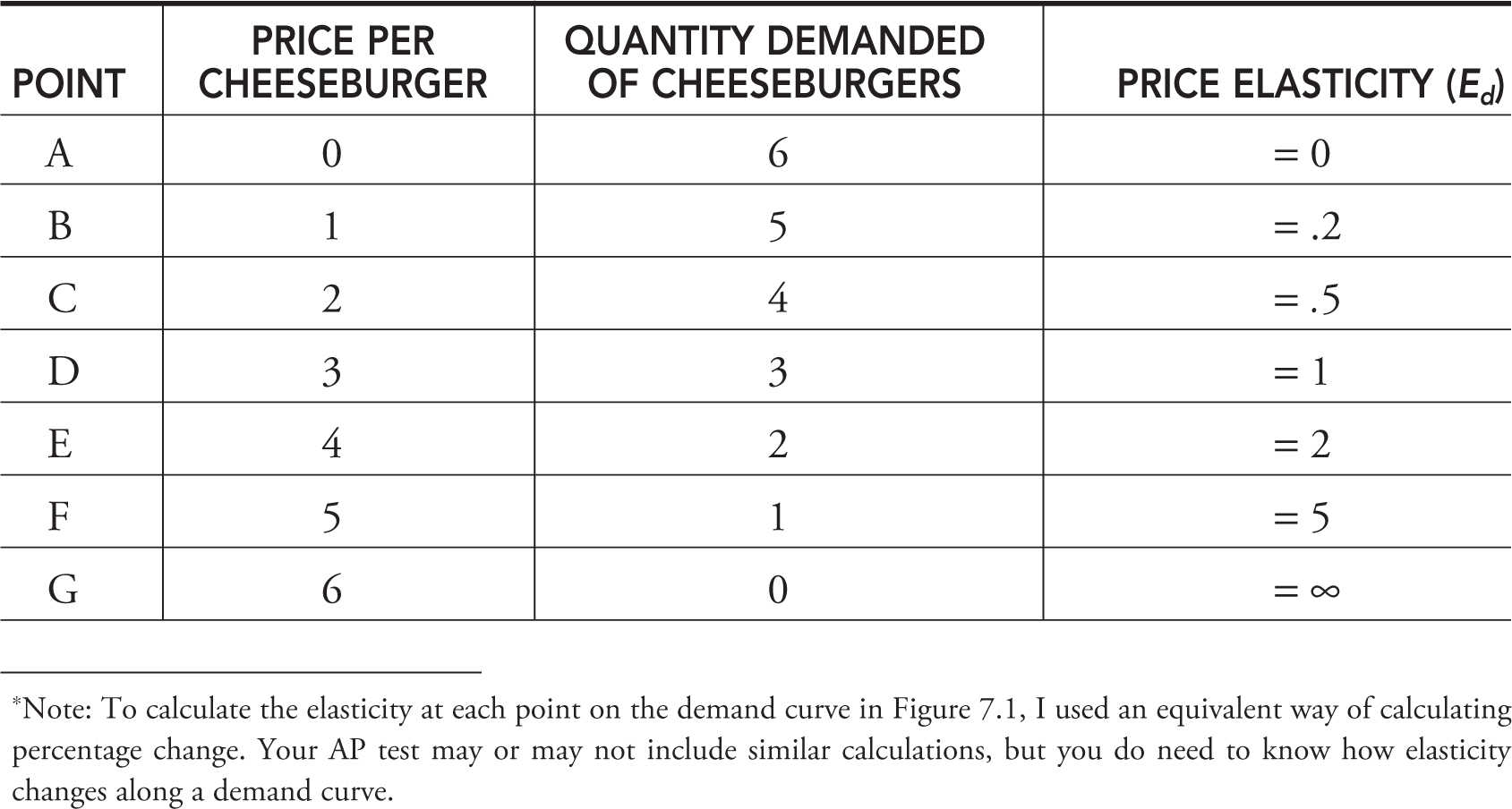
Elasticity on the Demand Curve

Take a very simple demand curve for cheeseburgers: P = 6 – Q _d , and plot this demand curve in Figure 7.1 .

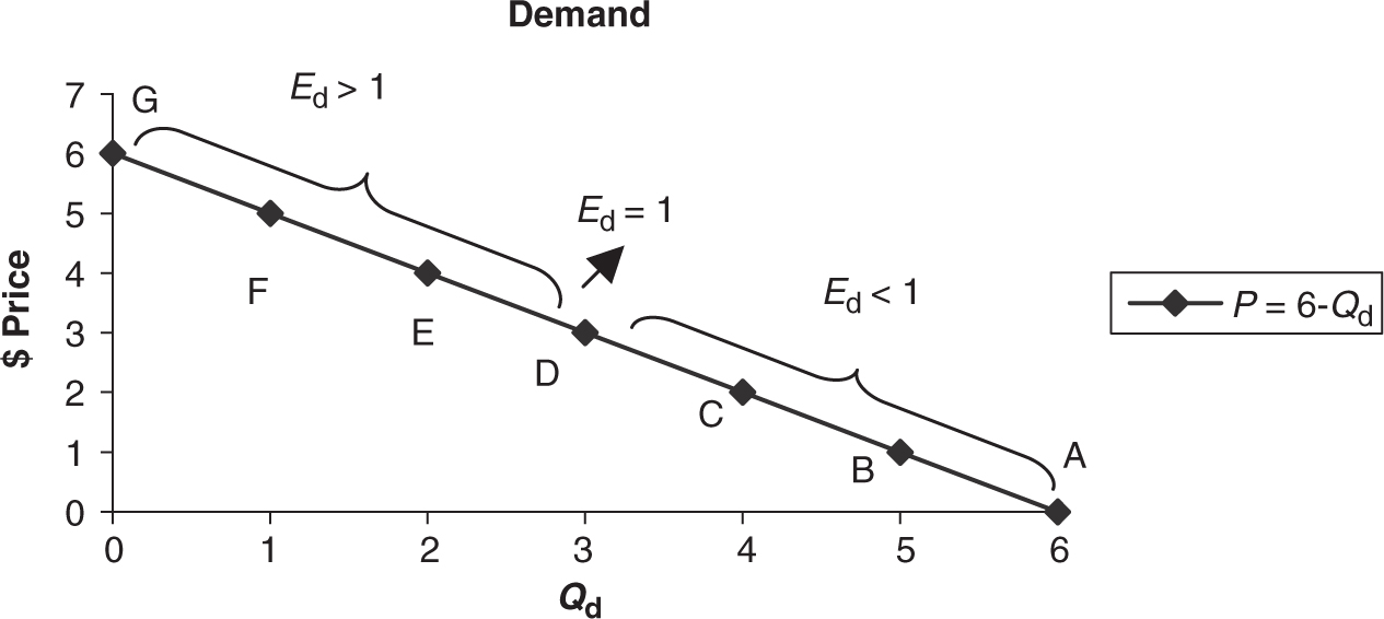
Figure 7.1

Table 7.1 summarizes changes in price, quantity demanded, and price elasticity at each point on the demand curve.*

As you can see in Figure 7.1 , the price elasticity of demand is not constant at points A through G on the demand curve. Specifically, as the price rises, E _d rises, telling us that consumers are more price sensitive at higher prices than they are at lower prices. This makes good intuitive sense. When the price is relatively low (e.g., point B), a 10 percent increase in price might be almost negligible to consumers. But if the original price is quite high (point F), then a 10 percent increase in the price is pretty drastic. In fact, if we divide the demand curve in half, you can see that above the midpoint (point D), demand is price elastic and below the midpoint, demand is price inelastic. At the midpoint, demand is unit elastic.

Table 7.1

The Midpoint Formula

Calculating the percentage change between two prices or quantities on a demand curve is not always easy; after all, the percentage change between two values depends on which of them is the initial value. For example, if a price increases from $100 to $125, this is a 25 percent increase. If the price falls from $125 to $100, this is a 20 percent decrease. The two prices on the demand curve are the same, but the percentage change between them depends on where we begin.

To avoid some of the difficulties of calculating these types of changes, we use what is known as the midpoint formula. Let’s use P ₁ and Q ₁ to represent the first point on the demand curve and P ₂ and Q ₂ to represent the second point. The midpoint formula calculates the price elasticity of demand between those two points by using the average price (P _avg ) and average quantity (Q _avg ) between them. The midpoint formula is therefore

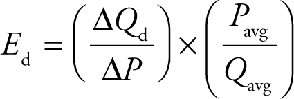
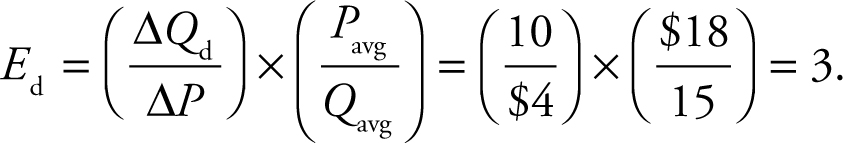
Let’s say that the initial price of a hypothetical product is $16, and 20 units are demanded. When the price rises to $20, quantity demanded falls to 10 units. The average price between these two points is $18, and the average quantity is 15 units. When we use the midpoint formula, we compute

Some recent AP Microeconomics exams have required the use of the midpoint formula, so it is important to be able to perform such calculations to maximize your free-response points.

Special Cases

If it is true that any increase in the price results in no decrease in the quantity demanded, then we are describing the special case where demand for the good is perfectly inelastic. Figure 7.2 shows the demand (D₀ ) for a life-saving pharmaceutical, for which there is no substitute, and without which the patient dies. The vertical demand curve tells us that no matter what percentage increase, or decrease, in price, the quantity demanded remains the same. Mathematically speaking, E _d = 0.

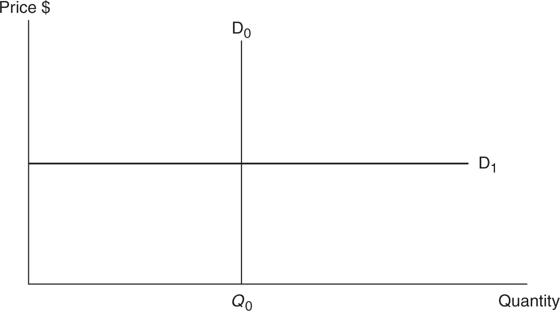
Figure 7.2

Figure 7.3

In the case where a decrease in the price causes the quantity demanded to increase without limits, then we have the special case where demand is perfectly elastic for that good. Figure 7.2 shows demand for a good (D₁ ), maybe one farmer’s grain, which has many substitutes. A horizontal demand curve tells us that even the smallest percentage change in price causes an infinite change in quantity demanded. Mathematically speaking, E _d = ∞.

Comparing the vertical (perfectly inelastic) demand curve to the horizontal (perfectly elastic) demand curve allows us to draw an important generalization. As a demand curve becomes more vertical, the price elasticity falls and consumers become more price inelastic. The opposite generalization can be made as the demand curve becomes more horizontal. Figure 7.3 illustrates some general points about slope and elasticity.

• In general, the more vertical a good’s demand curve (D₀ ), the more inelastic the demand for that good.

• The more horizontal a good’s demand curve (D₁ ), the more elastic the demand for that good.

• Despite this generalization, be careful; elasticity and slope are not equivalent measures.

Determinants of Elasticity

Perfectly elastic and perfectly inelastic demand curves are usually reserved for the hypothetical example, but they illustrate that E _d differs across consumer goods. Your intuition is that consumers respond to a price change in different ways. A 10 percent increase in the price of a car might have a drastically different consumer response from what we observe from a 10 percent increase in the price of a college education, a package of mechanical pencils, or a hotel stay in Fort Lauderdale. Let’s look at some general explanations for why elasticity differs.

1. Number of Good Substitutes

If the price of good X increases, and many substitutes exist, the decrease in quantity demanded can be quite elastic. For this reason, we expect E _d of orange juice to be high, since there are many substitutes available to drinkers of fruit juice.

Corollary . Oftentimes you hear of a good that is a “necessity” or a “frivolity.” These adjectives are reiterating a relative lack of or a relative wealth of good substitutes.

Example:

The more narrowly the product is defined, the more elastic it becomes. If we narrow our focus from orange juice down to one brand of orange juice (e.g., Minute Maid), the number of substitutes grows and we predict that so too does the price elasticity of demand for Minute Maid brand orange juice. Likewise, the demand for blue Chevrolet SUVs is more elastic than the demand for Chevrolet SUVs, which, in turn, is more elastic than the demand for all SUVs.

2. Proportion of Income

If the price of a good increases, the consumer loses purchasing power. If that good takes up a large proportion of the consumer’s income, he greatly feels the pinch of the income effect, and his responsiveness might be significant. If the price of toothpicks increased by 10 percent, the typical household probably would not feel the lost purchasing power and E _d would be low. The opposite would be true if the price of food items increased by 10 percent.

Example:

A young full-time college student is purchasing her education by the credit-hour and supporting herself with a part-time job on the weekends and evenings. Since the student is living on a relatively small monthly income, if the price of a credit-hour increases, the response might be very elastic. The student might drop down to part-time status or drop out of college altogether so that she can save enough money to return next quarter.

3. Time

Consumers faced by a rising price are usually fairly resourceful in their ability to find a way of decreasing the quantity demanded of a good. The difficulty faced by consumers is that they might not have time, at least not initially, to find a substitute for the more expensive good. We expect price elasticity to increase as more time passes after the initial increase in the price.

Example:

If the price of gasoline rises, consumers driving large SUVs do not immediately switch to small cars and the E _d is low for gasoline. But given enough time, if the gas price remains high, the E _d for gasoline increases.

Total Revenue and Elasticity

Discussing price elasticity and making simple calculations is not just a delightful academic exercise for students. Knowing how sensitive consumers are to changes in price is important to those who benefit from selling goods to those consumers—the sellers. Sellers compute total revenues collected from selling goods.

Total revenue = Price × Quantity demanded

A seller might think, “If I continue to raise the price, my total revenues must continue to rise.” A student of microeconomics knows that this is flawed logic, because quantity demanded falls when the price rises, making the impact on total revenue uncertain.

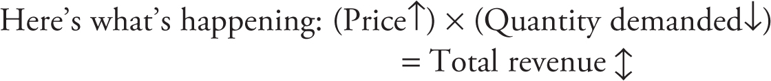
With price going up and quantity demanded going down, it’s like a tug-of-war between two teams, with total revenue being pulled in the direction of the strongest team.

Whether or not the total revenue increases with a price increase depends upon whether or not the gain from the higher price offsets the loss from lower quantity demanded. Price elasticity is an excellent way to predict how total revenue changes with a price change. This is sometimes called the total revenue test. Table 7.2 extends our earlier table by adding a column for total revenue at points A through G.

Table 7.2

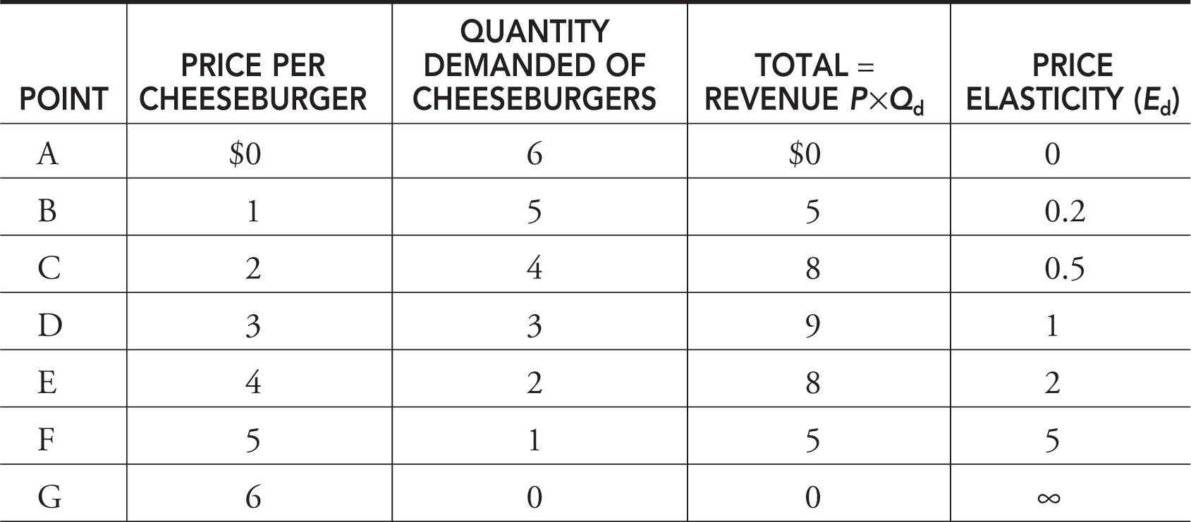
As you can see, if the price rises in the inelastic range of the demand curve, total revenues rise. However, if the price continues to rise into the elastic range, total revenues begin to fall. Why? Maybe a reminder of what it means for demand to be elastic helps to predict which team wins the tug-of-war.

• Inelastic demand E_d < 1: % ΔQ _d < % ΔP , so total revenue increases with a price increase.

• Elastic demand E_d > 1: % ΔQ _d > % ΔP , so total revenue decreases with a price increase.

• Unit elastic demand E _d = 1: % ΔQ _d = % ΔP , so total revenue remains the same.

In Figures 7.4 and 7.5 , we can graphically illustrate the connection between the demand curve, elasticity, and total revenue.

Income Elasticity of Demand

In the case of the income elasticity , it is a measure of how sensitive consumption of good X is to a change in a consumer’s income.

E_I = (% Δ Q _d good X)/(% Δ income)

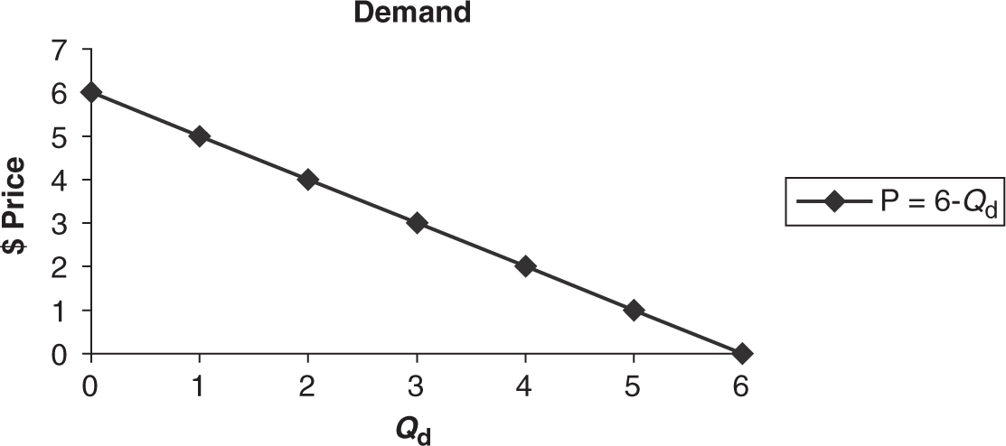
Figure 7.4

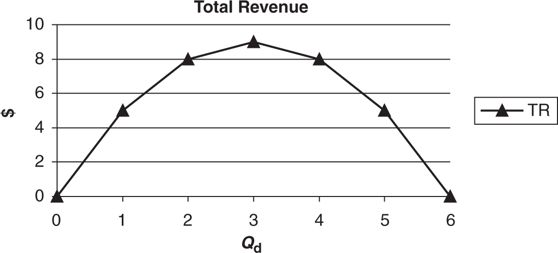
Figure 7.5

Example:

Jason’s income rises 5 percent, and we see his consumption of fast-food meals rises 10 percent.

E_I = 10%/5% = 2

So what do we make of this? First, because E_I is greater than zero, we can determine that fast-food meals are a normal good for Jason. Second, at least in this example, the consumption of fast-food meals is quite income elastic. A relatively small percentage increase in income causes a large—in fact, twofold—percentage increase in fast-food meals. Some refer to these goods as luxuries .

Example:

Jen’s income rises 5 percent, and we observe her consumption of bread rises 1 percent.

E_I = 1%/5% = .2

Once again, this measure would indicate that bread is a normal good, as more income prompts more bread consumption. However, the relatively small increase in consumption compared to the increase in income tells us that bread demand is relatively income inelastic. This makes sense; after all, how much more bread does one really wish to consume as his or her income rises? If Jen’s income doubled, would she double, or more than double, her consumption of bread? These goods are often referred to as necessities .

Example:

Consumer income increases by 5 percent, and we observe consumption of packaged bologna decreases by 2 percent.

E_I = –2%/5% = –.4

Again, there are two important observations that can be made here. First, because consumption of bologna decreased with an increase in income, we can conclude that bologna, in this example, is an inferior good. Second, there is a relatively inelastic response in bologna consumption to a change in income.

• If E_I > 1, the good is normal and income elastic (a luxury).

• If 1 > E_I > 0, the good is normal but income inelastic (a necessity).

• If E_I < 0, the good is inferior.

Cross-Price Elasticity of Demand

Consumers also change their consumption of good X when the price of a related good, good Y changes. The sensitivity of consumption of good X to a change in the price of good Y is called the cross-price elasticity of demand .

E_x,y = (%Δ Q _d good X)/(% Δ Price good Y)

Example:

The price of eggs increases by 1 percent, and the consumption of bacon falls 2 percent. The fact that bacon consumption fell when eggs became more expensive tells us that these goods are complementary goods.

E_x,y = (%Δ Q _d bacon)/(% Δ Price eggs) = –2%/1% = –2

Example:

The price of Honda cars increases 2 percent and consumption of Ford cars increases 4 percent. Because Ford cars saw increased consumption when Honda cars got more expensive, the two goods are substitutes.

E_x,y = (%Δ Q _d Ford)/(% Δ Price Honda) = 2%/1% = +2

• A cross-price elasticity of demand less than zero identifies complementary goods.

• A cross-price elasticity of demand greater than zero identifies substitute goods.

Price Elasticity of Supply

Now that we have addressed the sensitivity of consumer consumption of good X, let us discuss elasticity from the supplier’s perspective. When the price of good X changes, we expect quantity supplied to change. The law of supply predicts that as the price of good X increases, so too does quantity supplied. But what we do not know is, “by how much?” The price elasticity of supply helps to measure this response.

Price Elasticity of Supply Formula

E_s = (%Δ in quantity supplied of good X)/(% Δ in the price of good X)

Note: The law of supply ensures that E_s is positive. The greater this ratio, the more sensitive, or responsive, suppliers are to a change in the price of good X.

The Element of Time

Perhaps the most important determinant of how price elastic suppliers are in a particular industry is the time that it takes suppliers to change the quantity supplied once the price of the good itself has changed. This flexibility, of course, is different for different types of producers.

Example:

A local attorney produces hours of legal service in a small Midwestern town from her small office. At the current market price, for an hour of legal advice, she works a 40-hour workweek with the help of one clerical employee. If the price of an hour of legal assistance rises by 10 percent in the local market, initially our attorney responds by working a few additional minutes each weekday evening and on Saturday, but the constraints of the calendar allow for only an increase of 5 percent in the hours that she supplies.

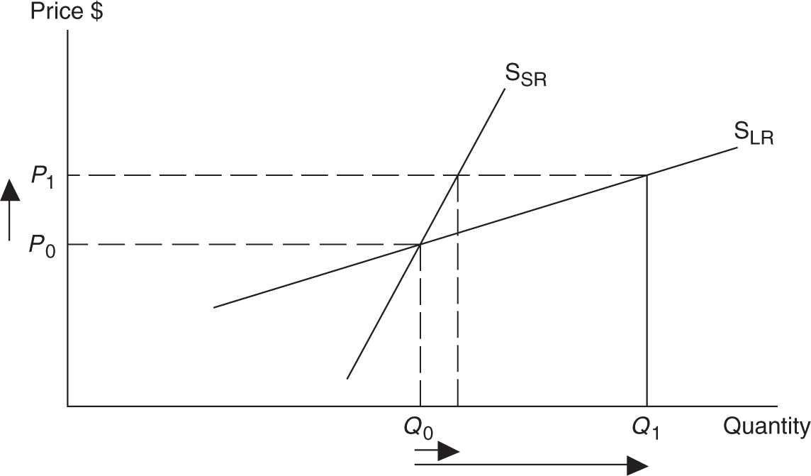
Figure 7.6

Short-term E_s = 5%/10% = .5

If this higher price is maintained for a month or two, the attorney might ask her employee to work additional hours, thus allowing the small office to increase the quantity of hours supplied by 10 percent. And if the price continues to stay at the higher rate, she might expand the office and employ a junior associate and thus increase the hours supplied by 20 percent.

Long-term E_s = 20%/10% = 2

Because suppliers, once the price of the good has changed, usually cannot quickly change the quantity supplied, economists predict that the price elasticity of supply increases as time passes. Figure 7.6 illustrates the short-term (S_SR ) and long-term (S _LR ) supply curves for our attorney. In general, the less steep the supply curve, the more elastic suppliers are in response to a change in the price.

7.2 Microeconomic Policy and Applications of Elasticity

Main Topics: Excise Taxes, The Role the Supply Curve Plays in the Impact of an Excise Tax, Subsidies, Price Floors, Price Ceilings

Excise Taxes

Government occasionally imposes an excise tax on the production of a good or service. Because it is a per unit tax on production, the firm responds as if the marginal cost of producing each unit has risen by the amount of the tax. Graphically this results in a vertical shift in the supply curve by the amount of the tax. The reasons for this tax are usually twofold: (1) to increase revenue collected by the government and/or (2) to decrease consumption of a good that might be harmful to some members of society. For these reasons, tobacco is a good example of an excise tax. Can an excise tax on tobacco raise money for government? Can it deter people from smoking? Let’s use our two extreme demand curves to see where these goals might, or might not, be achieved and how the price elasticity of demand plays a critical role on where the burden, or incidence , of the tax rests. Economists commonly express the incidence of the tax as the percentage of the tax paid by consumers, in the form of a higher price.

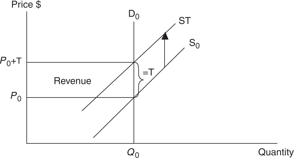
Figure 7.7

Demand Is Perfectly Inelastic

If the demand for cigarettes is perfectly inelastic (E _d = 0), then the demand curve (D ₀ ) is vertical. With an untaxed supply (S ₀ ) of cigarettes, the initial price of a pack of cigarettes is P ₀ and Q ₀ packs of cigarettes are consumed every day. If a per unit tax of T is imposed on the producers of cigarettes, the supply curve shifts upward by T . Be careful! This is not an “increase in supply”! Because the demand is perfectly inelastic, the equilibrium quantity remains at Q ₀ , but the new price rises to P ₀ + T . Total dollars spent on cigarettes increases from P ₀ × Q ₀ to (P ₀ + T ) × Q ₀ . The revenue collected by the government is equal to the area of the rectangle T × Q ₀ .

Did our excise tax accomplish our goals? Since quantity remained constant, the tax did nothing to decrease the harmful effects of smoking in society and only increased tax revenues for the government. In fact, because the quantity demanded did not fall, this scenario creates the largest revenue rectangle collected by the government. Who paid the burden of the tax? In Figure 7.7 , you can see that the entire tax was paid by consumers in the form of a new price exactly equal to the old price plus the tax.

Demand Is Perfectly Elastic

Figure 7.8 shows that if the demand for cigarettes is perfectly elastic (E _d = ∞), then the demand curve (D₀ ) is horizontal. With an untaxed supply (S₀ ) of cigarettes, the initial price of a pack of cigarettes is P ₀ and Q ₀ packs of cigarettes are consumed daily. The per unit tax of T shifts the supply curve upward by T , but with a perfectly elastic demand curve, the equilibrium price of cigarettes does not change, while equilibrium quantity demanded falls to Q₁ . Total spending by consumers falls to the area P ₀ × Q ₁ . Tax revenue for the government is a much smaller rectangle T × Q ₁ .

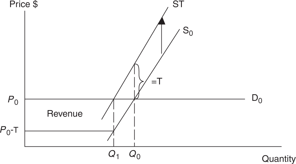
Figure 7.8

Who paid for the tax in this case? Because the price of a pack of cigarettes did not increase after the tax, it was not the consumers. Each producer receives a price of P ₀ but must then pay T to the government, so the net price received from each pack of cigarettes is (P ₀ – T ). So the producer pays the entire share of the tax when demand is perfectly elastic. Compared to the perfectly inelastic scenario, the government collected much fewer tax revenue dollars, but the maximum decrease in harmful cigarette consumption is a definite plus.

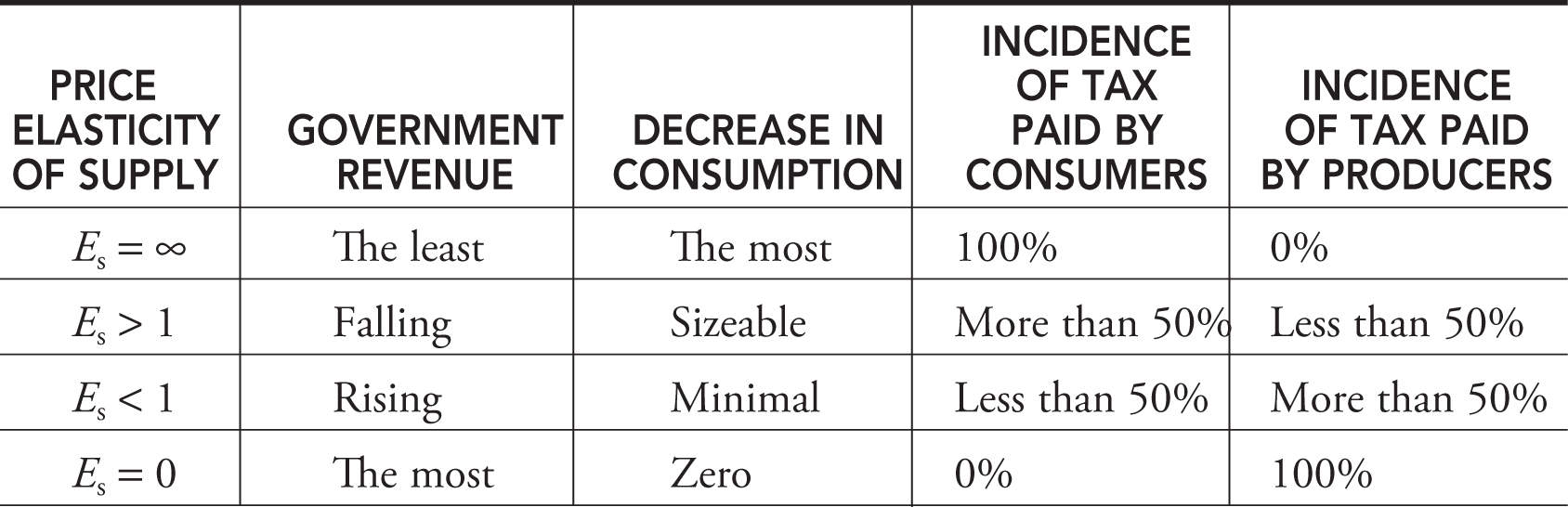
With these two extreme cases as benchmarks, we can conclude that as demand is more inelastic, consumers pay a higher share of an excise tax. Government revenues from the excise tax increase with inelastic demand, but the goal of decreasing consumption sees only minimal success. Table 7.3 summarizes the effects of a higher excise tax and how these depend upon the price elasticity of demand.

Table 7.3

Since cigarette demand is usually inelastic, significant improvements in the health of consumers is probably not the primary outcome of higher excise taxes, although they would seem to be effective revenue-generating devices. Ironically, although the tax is actually imposed on suppliers of cigarettes, most of the burden of the tax falls upon consumers. Figure 7.9 illustrates an inelastic demand for cigarettes, before and after an excise tax.

The Role the Supply Curve Plays in the Impact of an Excise Tax

We have seen that the greater the price elasticity of demand, the smaller the portion of the tax paid by consumers. It is also true that the price elasticity of supply plays a role in determining how much a tax will cause the price to increase and therefore helps to determine which group, consumers or producers, pays a higher burden of a tax.

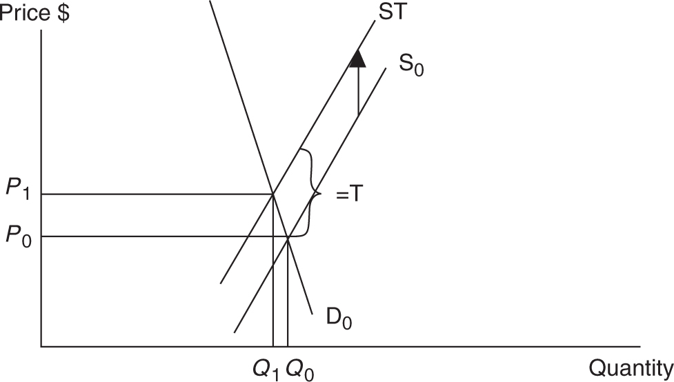
Figure 7.9

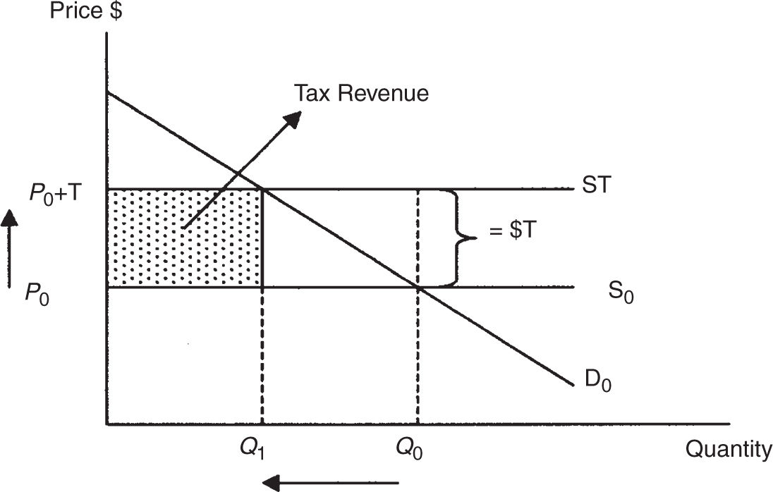
Figure 7.10

It again helps to see if we look at two extremes: a perfectly elastic supply curve and a perfectly inelastic supply curve.

A perfectly elastic, or horizontal, supply curve tells us that even a very small change in the price will cause an infinitely large change in the quantity supplied. A per unit tax T imposed on suppliers causes this horizontal supply curve to shift upward by the amount of the tax. In Figure 7.10 , you can see that the new equilibrium price is exactly T higher than the old price P ₀ , so consumers pay the entire burden of the tax. The equilibrium quantity decreases from Q ₀ to Q ₁ , and the government collects tax revenue equal to T × Q ₁ .

A perfectly inelastic, or vertical, supply curve illustrates the special case where any change in the price creates absolutely no change in quantity supplied. Figure 7.11 shows that in this case, the supply curve cannot vertically shift. At the equilibrium quantity Q ₀ , suppliers would like to charge a higher price than P ₀ , but any price above P ₀ creates a surplus, and this surplus will clear only at the equilibrium price P ₀ . Therefore the firms must pay T to the government for each of the Q ₀ units that are sold and consumers continue to pay the original price of P₀ . In this special case, producers pay the entire burden of the tax because, after paying the tax, they receive only (P ₀ – T ) on each unit. The government collects total revenue equal to T × Q ₀ .

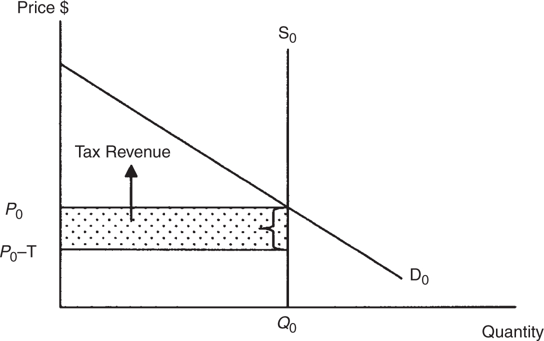
Figure 7.11

Table 7.4 summarizes the effects of a higher excise tax and how these depend upon the price elasticity of supply.

Table 7.4

By now you are probably wondering, “How can I keep all of this straight?” If we consider the extreme cases of perfectly elastic and perfectly inelastic demand and supply curves, we can draw some general conclusions.

• As the price elasticity of demand falls, and the price elasticity of supply rises, the greater the consumer’s share of a per unit excise tax. Why? Because this describes a situation where the consumer response to a higher price is negligible and the producer’s response is sizable. The group that has the best ability to respond to the higher post-tax price is going to make out better.

• Conversely, as the price elasticity of demand rises and the price elasticity of supply falls, the producer’s share of a per unit excise tax rises.

Loss to Society

There is also a cost to society when an excise tax is imposed on a competitive market. In the hypothetical soda market depicted in Figure 7.12 , the equilibrium quantity is 100 and the equilibrium price is $1. At this point, the marginal benefit to society exactly equals the marginal cost and net benefit; total welfare (combined consumer and producer surplus) is the greatest. When a $1 excise tax is imposed, the price of sodas paid by consumers increases to $1.80, and the number (amount) of sodas consumed decreases to 80. After sellers pay the excise tax, the price they receive falls to $0.80. The government collects $80 = $1 × 80 in tax revenue. With the tax, consumers and producers demand and supply 20 fewer units than without the tax. For these 20 units that go unproduced, the marginal benefit to consumers exceeds the marginal costs to producers. The fact that these 20 units go unproduced and unconsumed results in an inefficient outcome. The triangle labeled DWL used to be earned by society in the form of consumer and producer surplus. With the excise tax, society loses this area; it goes to no one. Economists call this area deadweight loss (DWL), or the net benefit sacrificed by society when such a per unit tax is imposed. Since the key to deadweight loss is a large decrease in quantity below the untaxed outcome, the area of dead-weight loss to society increases as the demand or supply curves get more elastic.

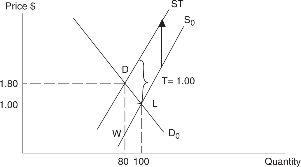
Figure 7.12

Note : Taxes such as these are not the only sources of distortions away from market efficiency. For example, production often generates pollution (a negative externality), which creates a situation where harmful spillover costs are incurred by third parties. Left unregulated, these costs are not captured by the market price and the market will not produce the “correct” amount of a good. These sources of inefficiency, or market failures, are addressed in Chapter 11 .

• Taxes create lost efficiency by moving away from the equilibrium market quantity where MB = MC to society.

• The area of deadweight loss (triangle DWL) increases as the quantity moves further from the competitive market equilibrium quantity.

Subsidies

A per unit subsidy on good X has the opposite effect of an excise tax, because firms respond as if the subsidy has lowered the marginal cost of production, therefore resulting in a downward vertical shift in the supply curve for good X. Be careful here! This is not a “decrease in supply”! Since subsidies come from the government, they are certainly not designed as revenue-generating devices. Ideally, their primary goal is to support producers of a good or service that has significant benefit to society so that it can be produced in greater quantities and at lower prices to consumers. This form of positive externality is also explored in Chapter 11 . Public university education is a common example of this type of subsidy.

Figure 7.13 illustrates the market for public university education where the demand (D ₀ ) and unsubsidized supply (S ₀ ) curves produce an equilibrium price P ₀ (tuition) and quantity Q ₀ (degrees earned). If government decides that provision of bachelor’s degrees is a beneficial service to society, a per student subsidy U is given to the public university system. The subsidy decreases tuition to P ₁ and increases the number of undergraduate degrees received. Notice that the producers receive, after the subsidy, (P ₁ + U ) for each student at the new quantity of Q ₁ .

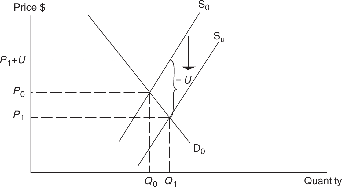
Figure 7.13

“Taxes and subsidies are usually tested in both the multiple-choice section and as part of a free-response question.”

—AP Teacher

How does the price elasticity of demand factor into this outcome? If the demand for public university education is elastic, then a relatively small percentage decrease in the price of tuition creates a sizable percentage increase in the number of degrees earned by members of society. If demand is price inelastic, it takes a much larger percentage decrease in the price to achieve the same percentage increase in degrees earned.

Price Floors

In some cases, the market-determined equilibrium price P ₀ is deemed “too low” by some members of society. Typically, suppliers who feel that the market price is not high enough to cover production costs and earn a decent living make this argument. If the government agrees with this argument, a price floor may be installed at some level above the equilibrium price. A price floor is a legal minimum price below which the product cannot be sold. Another example is a minimum wage in a market for labor. A price floor in the market for milk is seen in Figure 7.14 .

The resulting surplus of milk is not eliminated through the market, and the government usually agrees, as part of the price floor arrangement, to purchase the surplus milk. For consumers, the result of the policy is a higher price of milk (and other dairy products) at grocery stores, a decrease in milk consumption, and an increase in taxpayer-supported government spending. The amount of government spending to purchase the surplus is equal to (P _F ) × surplus. If the price elasticities of demand or supply are large, the surplus, and resulting government spending, rises.

By providing an incentive for producers to produce beyond where the MB = MC, the price floor policy causes efficiency to be lost. For gallons of milk above Q ₀ , MC > MB; there is an overallocation of resources to milk production. Quite simply, the policy produces a situation where “too much” milk is produced, and this is inefficient.

• A price floor is installed when producers feel the market equilibrium price is “too low.”

• A price floor creates a permanent surplus at a price above equilibrium.

• If the government purchases the surplus, taxpayers eventually pay the bill.

• The more price elastic the demand and supply curves, the greater the surplus and the greater the government spending to purchase the surplus.

• The price floor reduces net benefit by overallocating resources to the production of the good.

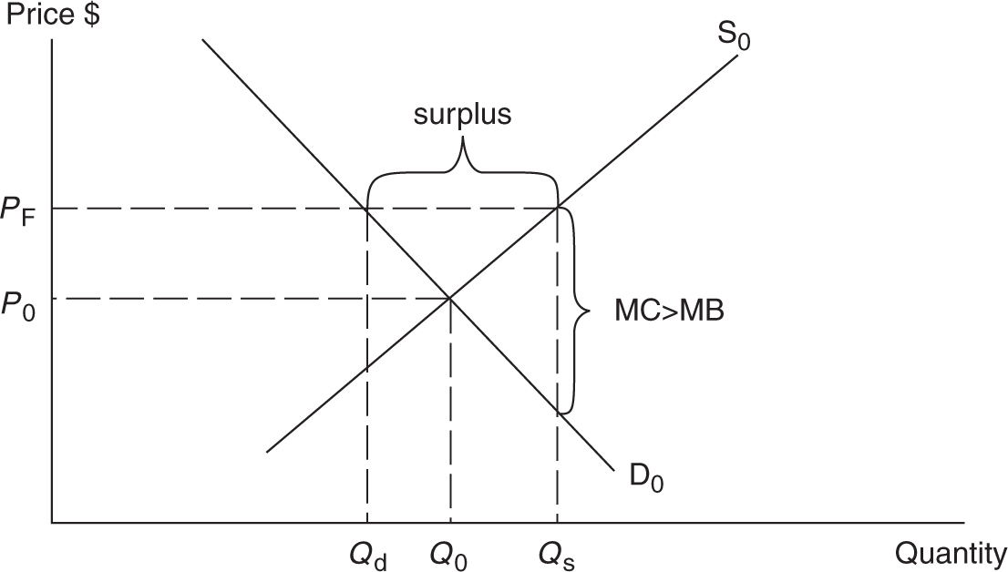
Figure 7.14

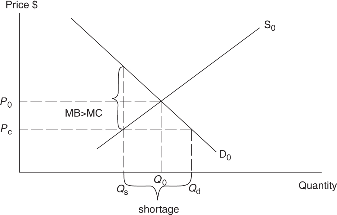
Figure 7.15

Price Ceilings

For some goods and services, the market equilibrium price is judged to be “too high.” Consumers who feel that the price is so high that it prevents a significant fraction of citizens from being able to consume a good, usually express this sentiment. If the government agrees with this argument, a price ceiling may be installed at a level below the equilibrium price. A price ceiling is a legal maximum price above which the product cannot be bought and sold. A price ceiling in the market for rental apartments (rent control) is seen in Figure 7.15 .

“Always remember on the graphs that floors are HIGH and ceilings are LOW.”

—Kristy, AP Student

The resulting shortage of rent-controlled apartments is not eliminated through the market, and this creates a sticky situation for low-income households, the group for which the policy was intended. Many suppliers completely remove their rental units from the market, converting them into office space or condominiums. Others attempt to increase profits by lowering levels of health and safety maintenance, or by charging exorbitant fees for a key to the apartment. For families lucky enough to find rent-controlled space, the result of this policy is certainly lower rents, but the shortage also tends to create an underground or “black” market for apartments where a vacant apartment might go to the highest bidder, regardless of financial need. If the price elasticities of demand or supply are large, the shortage, and the negative consequences of it, increase.

Again, this form of price control results in lost efficiency for society. When suppliers reduce their quantity supplied below the competitive equilibrium quantity, there is a situation where the MB > MC, and we see an underallocation of resources in the rental apartment market. This policy, intended to help low-income families, creates a situation where “too little” of the good is produced.

• A price ceiling is installed when consumers feel the market equilibrium price is “too high.”

• A price ceiling creates a permanent shortage at a price below equilibrium.

• The more price elastic the demand and supply curves, the greater the shortage.

• The price ceiling reduces net benefit by underallocating resources to the production of the good.

7.3 Trade Barriers

Main Topics: Tariffs , Quotas

The issue of free trade is hotly politicized. Proponents usually argue that free trade raises the standard of living in both nations , and most economists agree. Detractors argue that free trade, especially with nations that pay lower wages than those paid to domestic workers, costs domestic jobs in higher-wage nations. The evidence shows that in some industries, job losses have certainly occurred as free trade has become more prevalent. To protect domestic jobs, nations can impose trade barriers. Tariffs and quotas are among the most common of barriers.

Tariffs

In general, there are two types of tariffs. A revenue tariff is an excise tax levied on goods that are not produced in the domestic market. For example, the United States does not produce bananas. If a revenue tariff were levied on bananas, it would not be a serious impediment to trade, and it would raise a little revenue for the government. A protective tariff is an excise tax levied on a good that is produced in the domestic market. Though this tariff also raises revenue, the purpose of this tariff, as the name suggests, is to protect the domestic industry from global competition by increasing the price of foreign products.

Example:

The hypothetical domestic supply and demand for steel is pictured in Figure 7.16 . The domestic price is $100 per ton and the equilibrium quantity of domestic steel is 10 million tons. Maybe other nations can produce steel at lower cost. As a result, in the competitive world market, the price is $80 per ton. At that price, the United States would demand 12 million tons but only produce 8 million tons, and so 4 million tons are imported . It is important to see that in the competitive (free-trade) world market, consumer surplus is maximized and no deadweight loss exists. You can see the consumer surplus as the triangle below the demand curve and above the $80 world price.

If the steel industry is successful in getting a protective tariff passed through Congress, the world price rises by $10, increasing the quantity of domestic steel supplied and reducing the amount of steel imported from four million to two million tons. A higher price and lower consumption reduces the area of consumer surplus and creates deadweight loss.

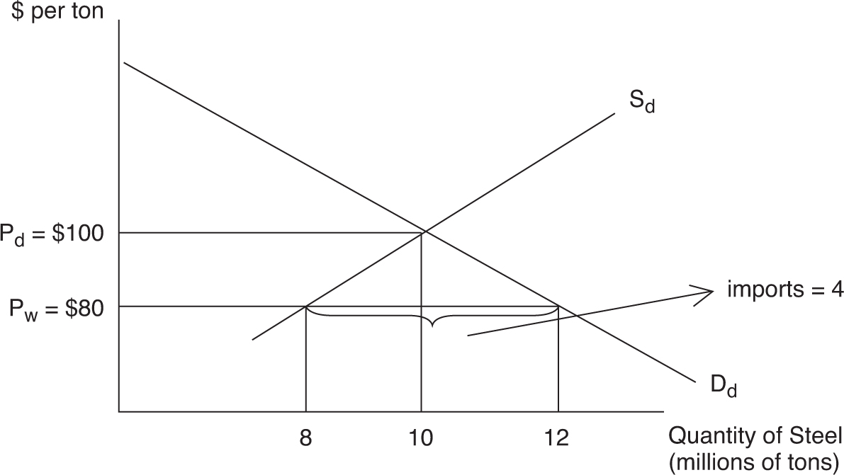
Figure 7.16

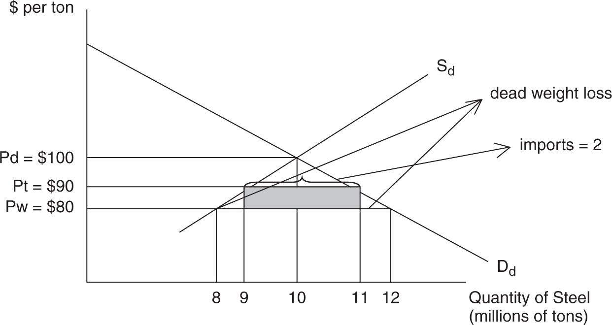
Figure 7.17

Economic Effects of the Tariff

• Consumers pay higher prices and consume less steel . If you are building airplanes or door hinges, you have seen an increase in your costs.

• Consumer surplus has been lost .

• Domestic producers increase output . Domestic steel firms are not subject to the tariff, so they can sell more steel at the price of $90 than they could at $80.

• Declining imports . Fewer tons of imported steel arrive in the United States.

• Tariff revenue . The government collects $10 × 2 million = $20 million in tariff revenue as seen in the shaded box in Figure 7.17 . This is a transfer from consumers of steel to the government, not an increase in the total well-being of the nation.

• Inefficiency . There was a reason the world price was lower than the domestic price. It was more efficient to produce steel abroad and export it to the United States. By taxing this efficiency, the United States promotes the inefficient domestic industry and stunts the efficient foreign sector. As a result, resources are diverted from the efficient to the inefficient sector.

• Deadweight loss now exists .

Quotas

Quotas work in much the same way as a tariff. An import quota is a maximum amount of a good that can be imported into the domestic market. With a quota, the government only allows two million tons to be imported. Figure 7.18looks much like Figure 7.17 , only without revenue collected by government. So the impact of the quota, with the exception of the revenue, is the same: higher consumer price and inefficient resource allocation.

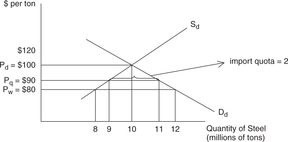
Figure 7.18

“It is important to know the differences between tariffs and quotas.”

—Lucas, AP Student

Tariffs and quotas share many of the same economic effects.

• Both hurt consumers with artificially high prices and lower consumer surplus.

• Both protect inefficient domestic producers at the expense of efficient foreign firms, creating deadweight loss.

• Both reallocate economic resources toward inefficient producers.

• Tariffs collect revenue for the government, while quotas do not.

7.4 Consumer Choice

Main Topics: Utility; Unconstrained Consumer Choice; Diminishing Marginal Utility; Constrained Utility Maximization; Constrained Utility Maximization Two Goods

Utility

If you pull back the curtain on the law of demand to study how consumers behave, much insight can be gained. It’s important to remember that people demand things because those things make those people happy . We choose to consume mundane items like electricity or crackers, or luxury items like trans-Atlantic flights and tickets to an NFL game, because they provide us with happiness. In economics, we call this happiness (or benefit, or satisfaction, or enjoyment) utility .

While in the course of a week, consumption of more and more pints of Cherry Garcia ice cream is likely to increase our total utility , it is probably safe to say that the first pint in a week provides more marginal utility than the second, third, or fourth pint. If you recall from Chapter 5 , analysis of marginal changes is extremely important in modeling how individuals make decisions.

• Total utility (TU) is the total amount of happiness received from the consumption of a certain amount of a good.

• Marginal utility (MU) is the additional utility received (or sometimes lost) from the consumption of the next unit of a good.

• Mathematically speaking: MU = ΔTU/ΔQ (this ΔQ is likely to equal 1 if you are consuming one additional unit at a time).

Example:

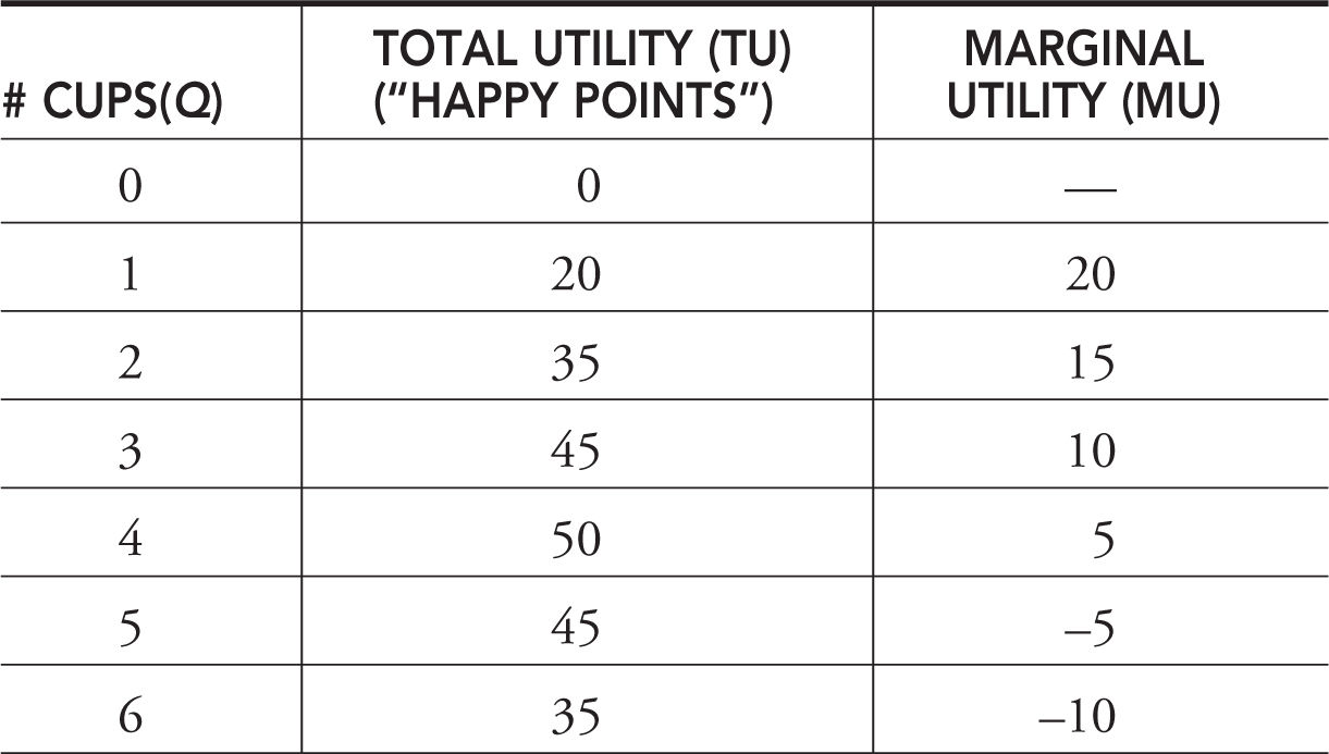
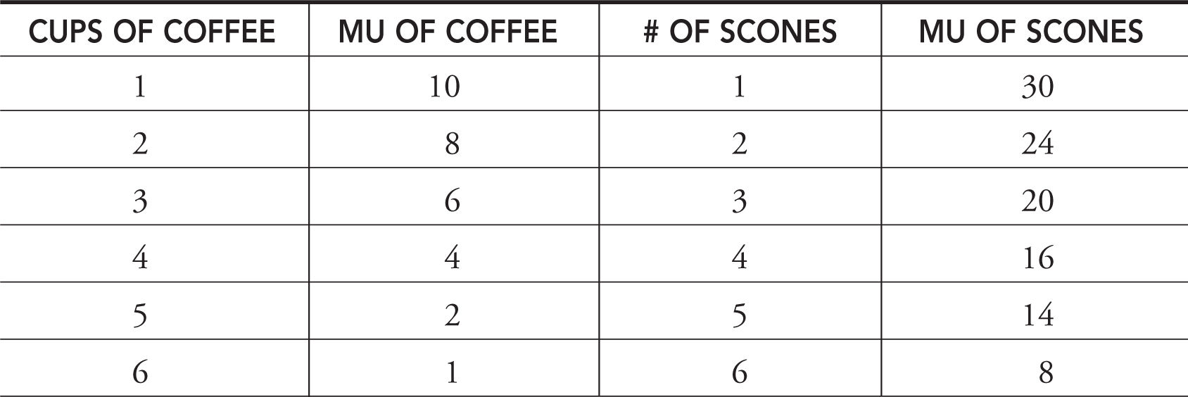
Table 7.5 summarizes the utility gained from consumption of successive cups of coffee in a typical morning at work. Some choose to measure utility in hypothetical “utils ,” but I like to think about these as “happy points.”

As our coffee drinker (Joe) goes from zero to one cup of coffee, his total happiness from coffee drinking increases from zero to 20 happy points. The incremental, or marginal, change is also 20 points. The marginal utility is simply calculated as the difference between the totals as Joe consumes consecutive cups of coffee.

Unconstrained Consumer Choice

So how much coffee should our desk jockey consume in a typical morning? Assuming that he does not have to pay for each cup and can freely use the coffee machine, one might assume that Joe consumes unlimited amounts of coffee. Using Table 7.5 or Figure 7.19 , you can easily see that total utility initially rises, peaks, and then begins to fall as more coffee is consumed. If Joe is a consumer who seeks to maximize happiness, and this seems a reasonable aim, he would not consume more than four cups of coffee, even if he were not asked to pay for each cup.

Table 7.5

• Even if the monetary price of good X is zero, the rational consumer stops consuming good X at the point where total utility is maximized.

Diminishing Marginal Utility

In Figure 7.19 you can see a relationship between total utility and coffee consumption. There is the obvious rise, peak, and fall of total utility as the number of cups increases. But closer inspection reveals that, as more coffee is consumed, total utility rises at a slower and slower rate. Since marginal utility is the rate at which total utility changes, marginal utility must be falling.

The law of diminishing marginal utility says that in a given time period, the marginal utility from consumption of one more of that item falls. A graphical depiction of marginal utility, also the slope of total utility, is seen in Figure 7.20 .

Constrained Utility Maximization

Now we require Joe to pay a price P_c for additional cups of coffee. With a fixed daily income and a price that must be paid, this individual is now a constrained utility maximizer . Joe must ask himself: “Does the next cup of coffee provide at least $P _c worth of additional happiness?” If Joe answers “yes” to this question for the first three cups of coffee, he maximizes his utility by stopping at three cups. If his answer is “no” to the fourth cup, he does not consume it.

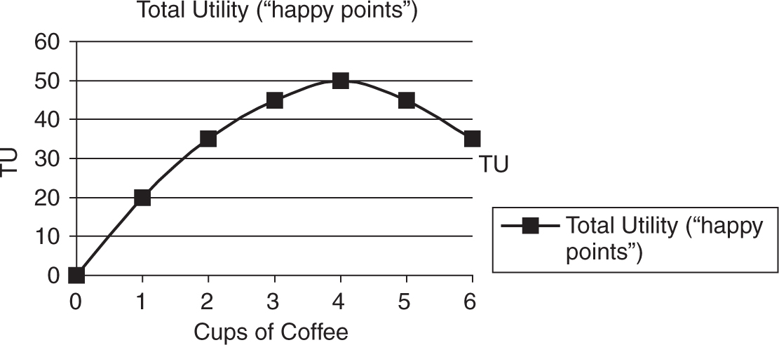
Figure 7.19

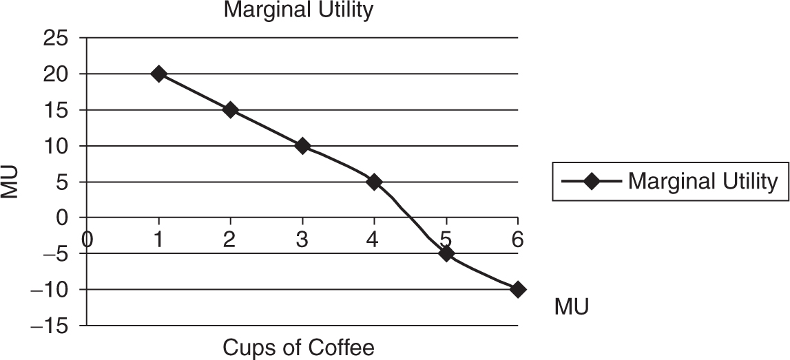
Figure 7.20

Does this sound familiar? It should, as it is another example of how a consumer never does something if the marginal benefit (in this case, utility) gained is exceeded by the marginal cost incurred.

• When required to pay a price, the utility maximizing consumer stops consuming when MB = P .

• This MB also represents the highest price, or “willingness to pay,” our consumer would be willing to pay for the next cup.

Demand Curve Revisited

Using the logic outlined above as an example, what would happen if the price of coffee fell? If Joe was facing a new lower price, you should expect that Joe would rationally increase his daily consumption of cups of coffee. Have you heard this behavior described before? Sure! It’s the law of demand, and it has a tight connection to the law of diminishing marginal utility.

Imagine you are a consumer who has already paid for and consumed the first pint of ice cream this week. Would your willingness to pay for the second pint of ice cream be the same as your willingness to pay for the first pint? Doubtful, because the second pint does not provide the same marginal utility as the first. In order to entice you to purchase and consume additional pints of Cherry Garcia ice cream, the price must fall to compensate you for your falling marginal utility.

This law of diminishing marginal utility is the backbone of the law of demand. To convert the relationship between marginal utility and quantity consumed at any price, we might ask you how much you are willing to pay to consume successive pints of ice cream. Because of diminishing marginal utility, you offer to pay less for additional units. Thus, we can then construct your monthly demand curve for ice cream. Figure 7.21 illustrates how diminishing marginal utility from consumption of a good can be converted to a demand curve for that good.

Constrained Utility Maximization, Two Goods

Economists see a consumer, constrained by income and prices, as living within a budget constraint. In a simple case where one good is consumed, the consumer maximizes utility by buying units of good X up to the point where the marginal utility of the last unit of good X is equal to the price. Most consumers allocate limited income between many goods and services, each with a price that must be paid. To see how a consumer maximizes utility in this situation, we consider a two-good case where, in addition to daily cups of coffee, Joe also purchases scones. We start with a “rule” and then proceed to solve a couple of problems.

“Learn the definitions first. This will make the logic much more obvious.”

—David, AP Student

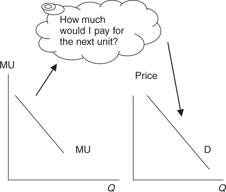
Figure 7.21

Utility Maximizing Rule

Given limited income, consumers maximize utility when they buy amounts of goods X and Y so that the marginal utility per dollar spent is equal for both goods. Another way to think about it is that they seek the most “bang for their bucks.” Mathematically, this utility maximizing rule is expressed

MU _x /P_x = MU _{y /} P_y or MU _x /MU _y = P_x /P_y

If the consumer has used all income and the above ratios are equal, they are said to be in equilibrium. Under this condition, no other combination of X and Y provides more total utility.

Example:

Joe has daily income of $20, each cup of coffee costs P_c = $2 and each scone costs P_s = $4. Table 7.6 provides us with Joe’s marginal utility received in the consumption of each good.

Table 7.6

• It is very important to remember that consuming more of one good causes the marginal utility to fall, but the total utility to rise.

In order to maximize Joe’s utility, he seeks a combination of coffee and scones so that MU _c /$2 = MU_s /$4 and spends exactly his income of $20. Another way to solve this problem is to rearrange these ratios so that:

MU _c /MU _s = $2/$4 = .5

There are several combinations of coffee and scones in Table 7.6 where the ratio of marginal utilities is one-half. For example, Joe could consume one cup of coffee (MU = 10) and three scones (MU = 20) for a total utility of 84 (10 + 30 + 24 + 20). But this combination would only spend a total of $14, and surely Joe would be happier if he used all of his income.

• To find the total utility of consuming cups of coffee, sum up the marginal utility of each cup consumed. Do the same for scones to calculate total utility.

Another possibility is to consume two cups of coffee (MU = 8) with four scones (MU = 16). This does indeed spend exactly $20. The total utility of 108 confirms that Joe is happier with this combination of coffee and scones. There exists one other combination of goods that satisfies our rule: four cups of coffee (MU = 4) with six scones (MU = 8) expends too much money ($32) for Joe’s income.

So according to our rule, Joe’s utility maximizing decision would be to use his income of $20 to consume two cups of coffee and four scones. What if he decided to experiment and reallocate his consumption while still spending only $20 on coffee and scones? For example, four cups of coffee (MU = 4) and three scones (MU = 20) fails our rule, but Joe still is spending $20. On closer inspection, this is a poor decision because total utility falls to 102.

Example:

Now the price of a cup of coffee falls to $1. Joe needs to reexamine his utility maximizing combination of coffee and scones.

MU _c /MU _s = $1/$4 = .25

Again, there are three possibilities, but only one uses exactly $20 of income. If Joe buys four cups of coffee (MU = 4) and four scones (MU = 16), he spends exactly his income and receives total utility of 118. The combination of three cups of coffee and two scones does not use all of the income, and the combination of five cups of coffee and six scones exceeds the income constraint.

Connection Back to Demand Curves

Joe, as a utility maximizing consumer, chooses two cups of coffee at a price of $2 and four cups of coffee at a price of $1. This sounds familiar! What Joe has done, simply by responding in a utility maximizing way, is illustrate the law of demand. The two combinations of price and quantity demanded are two points on Joe’s coffee demand curve. By connecting these points, we trace out his demand curve (Figure 7.22 ).

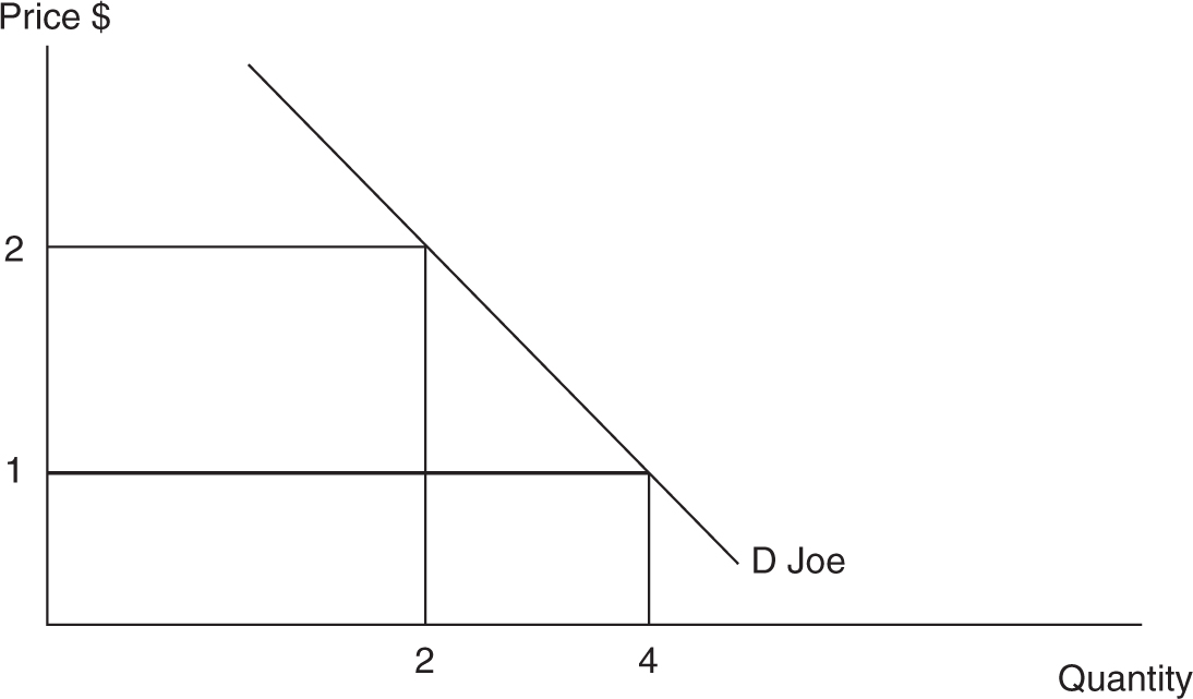
Figure 7.22

Individual and Market Demand Curves

We can take the individual decisions made by consumers like Joe and expand the analysis to build a market demand curve for coffee and other goods. This process is called horizontal summation . At every price, we would simply add the quantity demanded for all individual consumers.

• Utility maximizing behavior of individuals creates individual demand curves.

• Summing the quantity demanded by individuals at each price creates market demand curves.

Review Questions

1 . If the price of corn rises 5 percent and the quantity demanded for corn falls 1 percent, then

(A) E _d = 5 and demand is price elastic.

(B) E _d = 1/5 and demand is price elastic.

(C) E _d = 5 and demand is price inelastic.

(D) E _d = 1/5 and demand is price inelastic.

(E) E _d = 5 and corn is a luxury good.

2 . A small business estimates price elasticity of demand for the product to be 3. To raise total revenue, owners should

(A) decrease price as demand is elastic.

(B) decrease price as demand is inelastic.

(C) increase price as demand is elastic.

(D) increase price as demand is inelastic.

(E) do nothing; they are already maximizing total revenue.

3 . Mrs. Johnson spends her entire daily budget on potato chips, at a price of $1 each, and onion dip at a price of $2 each. At her current consumption bundle, the marginal utility of chips is 12 and the marginal utility of dip is 30. Mrs. Johnson should

(A) do nothing; she is consuming her utility maximizing combination of chips and dip.

(B) increase her consumption of chips until the marginal utility of chip consumption equals 30.

(C) decrease her consumption of chips until the marginal utility of chip consumption equals 30.

(D) decrease her consumption of chips and increase her consumption of dip until the marginal utility per dollar is equal for both goods.

(E) increase her consumption of chips and increase her consumption of dip until the marginal utility per dollar is equal for both goods.

4 . A consequence of a price floor is

(A) a persistent shortage of the good.

(B) an increase in total welfare.

(C) a persistent surplus of the good.

(D) elimination of deadweight loss.

(E) an increase in quantity demanded and a decrease in quantity supplied.

Use the figure below to respond to the next two questions.

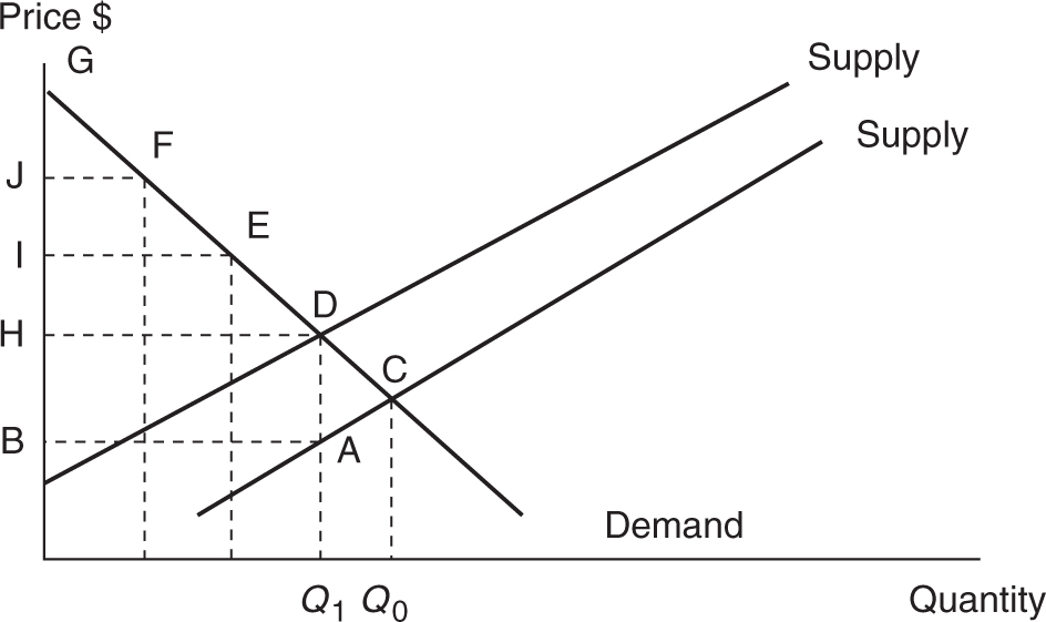
5 . The competitive market equilibrium is at point C. If a per unit excise tax is imposed on the production of this good, the deadweight loss is

(A) the area BDE.

(B) the area BADH.

(C) the area GDH.

(D) the area DAC.

(E) the area GDAB.

6 . The competitive market equilibrium is at point C. If a per unit excise tax is imposed on the production of this good, the revenue collected by the government is

(A) the area BDE.

(B) the area BADH.

(C) the area GDH.

(D) the area DAC.

(E) the area GDAB.

1 . D —You must know the formula for elasticity: E _d = (%ΔQ _d )/(%ΔP ) = 1/5. Since E _d < 1, this is inelastic demand, and you can quickly eliminate any reference to elastic demand. Although calculators are not allowed on the AP exam, simple calculations can be made in the margins of your exam.

2 . A —If you know your elasticity measures, you see that with E _d = 3, you can eliminate any reference to inelastic demand. Choice E is incorrect, as total revenue is maximized at the midpoint of the demand curve where E _d = 1. If E _d > 1, the firm increases total revenue by decreasing the price because the quantity demanded rises by a greater percentage than the fall in price.

3 . D —Mrs. Johnson needs to find the combination of chips and dip where the ratio of marginal utility per dollar is equated. Currently, MU_c /P_c = 12 and MU _d /P_d = 15, so choice A is ruled out. Since she is receiving more “bang for her buck” from dip consumption, she increases dip consumption and therefore decreases chip consumption. MU _d falls and MU _c rises. She adjusts her spending until MU _c /P_c = MU_d /P_d .

4 . C —Price floors are installed when the market equilibrium price is believed to be “too low.” This price lies above the equilibrium price, decreasing Q_d and increasing Q_s , thus creating a surplus. Price controls worsen total welfare and create deadweight loss.

5 . D —Deadweight loss is total welfare that used to be gained by society prior to the tax. When looking for deadweight loss, narrow your focus by comparing the quantity produced with and without the tax. The horizontal distance between Q ₀ and Q ₁ is the unattained output from the tax. The vertical distance between points D and A illustrates that the MB > MC and is therefore an inefficient outcome.

6 . B —Revenue collected by the government is equal to the per unit tax multiplied by the new quantity. The vertical distance between supply curves is the tax.

Rapid Review

Elasticity: Measures the sensitivity, or responsiveness, of a choice to a change in an external factor.

Price elasticity of demand ( E _d ): Measures the sensitivity of consumer quantity demanded for good X when the price of good X changes.

Price elasticity formula: E _d = (%ΔQ _d )/(%ΔP ). Ignore the negative sign.

Price elastic demand: E _d > 1 or the (%ΔQ _d ) > (%ΔP ). Consumers are price sensitive.

Price inelastic demand: E _d < 1 or the (%ΔQ _d ) < (%ΔP ). Consumers are not price sensitive.

Unit elastic demand: E _d = 1 meaning the (%ΔQ _d ) = (%ΔP ).

Perfectly inelastic: E _d = 0. In this special case, the demand curve is vertical and there is absolutely no response to a price change.

Perfectly elastic: E _d = ∞. In this special case, the demand curve is horizontal meaning consumers have an instantaneous and infinite response to a price change.

Slope and elasticity: In general, the more vertical a good’s demand curve, the more inelastic the demand for that good. The more horizontal a good’s demand curve, the more elastic the demand for that good. Despite this generalization, be careful, as elasticities and slopes are not equivalent measures.

Determinants of elasticity: If a good has more readily available substitutes (luxuries vs. necessities), it is likely that consumers are more price elastic for that good. If a high proportion of a consumer’s income is devoted to a particular good, consumers are generally more price elastic for that good. When consumers have more time to adjust to a price change, their response is usually more elastic.

Total revenue: TR = P × Q _d

Total revenue test: Total revenue rises with a price increase if demand is price inelastic and falls with a price increase if demand is price elastic.

Elasticity and demand curves: At the midpoint of a linear demand curve, E _d = 1. Above the midpoint demand is elastic and below the midpoint demand is inelastic.

Income elasticity: A measure of how sensitive consumption of good X is to a change in the consumer’s income.

Income elasticity formula: E_I = (%ΔQ _d good X)/(%Δ income)

Luxury: A good for which the income elasticity is greater than one.

Necessity: A good for which the income elasticity is above zero but less than one.

Values of Income Elasticity: If E_I > 1, the good is normal and a luxury. If 1 > E_I > 0, the good is normal and income inelastic (necessity). If E_I < 0, the good is inferior.

Cross-price elasticity of demand: A measure of how sensitive consumption of good X is to a change in the price of good Y.

Cross-price elasticity formula: E_x,y = (%ΔQ _d good X)/(%Δ price Y)

Values of cross-price elasticity of demand: If E_x,y > 0, goods X and Y are substitutes. If E_x,y < 0, goods X and Y are complementary.

Price elasticity of supply: Measures the sensitivity of quantity supplied for good X when the price of good X changes.

Price elasticity of supply formula: E _s = (%ΔQ _s )/(%ΔP )

Excise tax: A per unit tax on production results in a vertical shift upward in the supply curve by the amount of the tax.

Incidence of Tax: The proportion of the tax paid by consumers in the form of a higher price for the taxed good is greater if demand for the good is inelastic and supply is elastic.

Deadweight Loss: The lost net benefit to society caused by a movement away from the competitive market equilibrium. Policies like excise taxes create lost welfare to society.

Subsidy: Has the opposite effect of an excise tax, as it has the effect of lowering the marginal cost of production, resulting in a downward vertical shift in the supply curve for good X.

Price floor: A legal minimum price below which the product cannot be sold. If a floor is installed at some level above the equilibrium price, it creates a permanent surplus.

Price ceiling: A legal maximum price above which the product cannot be sold. If a ceiling is installed at a level below the equilibrium price, it creates a permanent shortage.

Utility: Happiness, benefit, satisfaction, or enjoyment gained from consumption.

Total utility: Total happiness received from consumption of a number of units of a good.

Marginal utility: The incremental happiness received, or lost, when the consumer increases consumption of a good by one unit.

Utils: A unit of measurement often used to quantify utility. Also known as “happy points.”

Law of diminishing marginal utility: In a given time period, the marginal (additional) utility from consumption of more and more of that item falls.

Constrained utility maximization: For a one-good case. Constrained by prices and income, a consumer stops consuming a good when the price paid for the next unit is equal to the marginal benefit received.

Utility maximizing rule: The consumer maximizes utility when they choose amounts of goods X and Y, with their limited income, so that the marginal utility per dollar spent is equal for both goods. Mathematically: MU _x /P_x = MU_y /P _y , or MU _x /MU _y = P _x /P _y .

Horizontal summation: The process of adding, at each price, the individual quantities demanded to find the market demand curve for a good.

Revenue tariff: An excise tax levied on goods not produced in the domestic market.

Protective tariff: An excise tax levied on a good that is produced in the domestic market so that it may be protected from foreign competition.

Import quota: A limitation on the amount of a good that can be imported into the domestic market.