5 Steps to a 5: AP Microeconomics 2017 (2016)
STEP 4
Review the Knowledge You Need to Score High
CHAPTER 8
The Firm, Profit, and the Costs of Production
IN THIS CHAPTER
Summary: The previous chapter focused on the choices made by consumers and how external forces and microeconomic policies affected those choices. The chapter concluded with the concept of constrained utility maximization and the utility maximizing rule. Also known as the consumer’s equilibrium, it goes a long way toward explaining demand for goods and services. This chapter examines much of the same but for firms, who are assumed to maximize profit by hiring the perfect combination of production inputs at the lowest cost. First the firm is introduced, along with the importance of opportunity costs and the economic view of profits. Then the short-run production function and several principles that flow from production are introduced. The discussion then turns to the short-run costs of employing inputs and important principles associated with costs. In particular, these concepts provide the foundation for the supply curve. Lastly, the analysis is extended into the long run.

Key Ideas
![]() Economic Profit
Economic Profit
![]() Short Run versus Long Run
Short Run versus Long Run
![]() Production in the Short Run
Production in the Short Run
![]() Law of Diminishing Marginal Returns
Law of Diminishing Marginal Returns
![]() Costs in the Short Run
Costs in the Short Run
![]() Costs in the Long Run
Costs in the Long Run
8.1 Firms, Opportunity Costs, and Profits
Main Topics: The Firm, Profit and Cost: When CPAs and Economists Collide, Short-Run and Long-Run Decisions
The Firm
When we talk about consumers, it’s very easy to imagine yourself in the leading role. However, when the conversation switches to the firm, it is often much more difficult to visualize what it is or who we are talking about. The firm can bring to mind many things to many different people. The firm can be an independent bookstore in your town, or it can be Barnes & Noble. It can be a street vendor selling hot dogs, or it can be Oscar Mayer. Regardless of the size of the business, a firm is defined as: “An organization that employs factors of production to produce a good or service that it hopes to profitably sell.”
Profit and Cost: When CPAs and Economists Collide
Before we launch into a technical discussion of production and costs, we need to take care of, well, a technicality. The bottom line is that the accountant sees profit differently than does the economist.
Example:
Upon completion of her undergraduate double major in accounting and economics, Molly creates a firm that sells lemonade on a busy street corner in her small town. Selling cups of lemonade at $1 each, Molly sells 1,000 cups per month. The accountant and the economist in her agree (imagine a little devil and little angel on each shoulder—you can decide which is the CPA) that monthly total revenues (TR) = $1 × 1,000 cups = $1,000.
Molly’s accounting textbooks clearly state that profit (π) is calculated by subtracting total production costs (TC) from total revenue. She rents a table from her parents at $75 per month; spends $300 per month on lemons, sugar, and cups; and purchases a monthly vendor’s license at $25. These direct, purchased, out-of-pocket costs are referred to as accounting costs, or explicit costs .

The economist on Molly’s other shoulder disagrees. Are these the only costs of running the lemonade stand? What about the opportunity costs of resources not accounted for above? For example, Molly has chosen to give up a monthly salary of $1,000 at a bank. The economist knows that this opportunity cost must be subtracted from total revenue to better measure profitability. These indirect, non-purchased, opportunity costs are called economic costs, or implicit costs .

Other implicit costs borne by many entrepreneurs include the interest given up when savings are liquidated, or rent forgone if the individual works out of a home or garage.
Here’s one way to try to keep explicit and implicit costs straight:
• Were the dollars paid to outside resource suppliers (employees, a landlord, a wholesale food store)? Did money actually change hands? Explicit .
• Were the resources supplied by the entrepreneur herself (salary or interest given up)? Implicit .
So Which Should I Use?
This is an excellent question. The “quickie” answer is to turn to the title page of this book, and use that method. Of course, as a student of economics, you must include implicit economic costs in calculating economic profit. But why? Well, it’s more accurate. An adept student of economics knows that the cost of something goes beyond the price tag. A friend of mine in graduate school once said that “nothing is free; it is just non-priced.” If you visit your AP teacher’s office, you might not have to pay to pass through the door, but you could be doing something else with your time. This is a non-priced economic cost. Molly’s labor and effort at the lemonade stand appear to be free; this is why an accountant does not include that effort in calculating profit. An economist knows that it is not free—it is just non-priced. An economist tries to quantify that price by using the value of Molly’s efforts in her next best alternative as the banker. Throughout this book, costs refer to economic costs, and profits refer to economic profits.
Short-Run and Long-Run Decisions
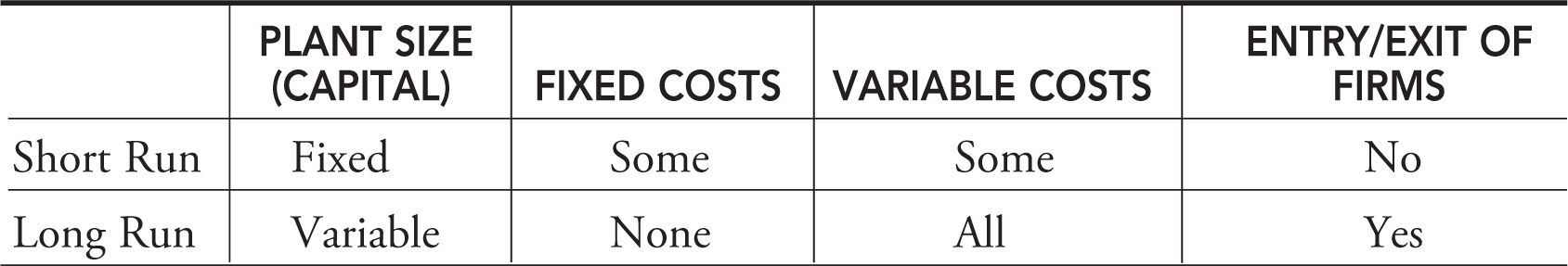
The short run is a time when at least one production input is fixed and cannot be changed to respond to a change in product demand. During the holiday season a local gift shop extends hours and increases the workers hired. Much more difficult to change is the total capacity of the shop. The capacity of the shop is fixed in the short run but can be altered with enough time. The amount of time required to change the plant size is known as the long run . In other words, all inputs are variable in the long run. See Table 8.1 .
Table 8.1
Example:
When Molly pays $25 for a monthly vendor’s license on January 1, she is committed for a month. She cannot receive a refund if she fails to operate the lemonade stand, and she does not have to pay more if she works 24 hours a day all month. For Molly, the long run is one month. On the other hand, at any point in the month, Molly can choose to purchase more lemons, cups, or sugar, or employ assistants if she is selling more cups of lemonade. This is a short-run decision.
8.2 Production and Cost
Main Topics: Short-Run Production Functions, Law of Diminishing Marginal Returns, Short-Run Costs, Bridge over (Troubling) Economic Waters, Long-Run Costs, Economies of Scale
Short-Run Production Functions
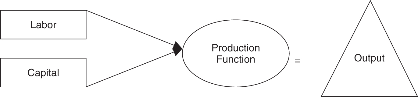
How do economic resources like labor, capital, natural resources, and entrepreneurial talent become a cup of lemonade, or a ton of copper, or a 30-second television commercial? A production function is the mechanism for combining production resources, with existing technology, into finished goods and services. In other words, a production function takes inputs and creates output. In a production function that uses only labor (L) and capital (K):
Fixed and Variable Inputs
The short run is a period of time too brief to change the plant capacity. This implies that some production inputs cannot be changed in the short run. These are fixed inputs . During the short run, firms can adjust production to meet changes in demand for their output. This implies that some inputs are variable inputs . Using only labor and capital, we assume that labor can be changed in the short run, but capital (i.e., the plant capacity) is fixed.
Short-Run Production Measures
By its very nature, production lends itself to be quantified, and as a result, you need to study these three production measures. To keep it simple, capital is assumed to be fixed while labor can be changed to produce more or less output.
1. Total product (TP L ) of labor is the total quantity, or total output, of a good produced at each quantity of labor employed.
2. Marginal product (MP L ) of labor is the change in total product resulting from a change in the labor input. MPL = ΔTPL /Δ L. If labor is changing one unit at a time, MPL = ΔTPL .
3. Average product (AP L ) of labor is also a measure of average labor productivity and is total product divided by the amount of labor employed: APL = TPL /L.
As you can see, MPL and APL are both derived from TPL . It is useful to see how these three measures are related with a numerical example.
Example:
In the production period of a month, Molly’s lemonade stand combines variable inputs of her labor (and the raw materials) to the fixed inputs of her table and her license to operate. Molly adds employees to her plant and forecasts the change in production (cups per day) in Table 8.2 .
Table 8.2
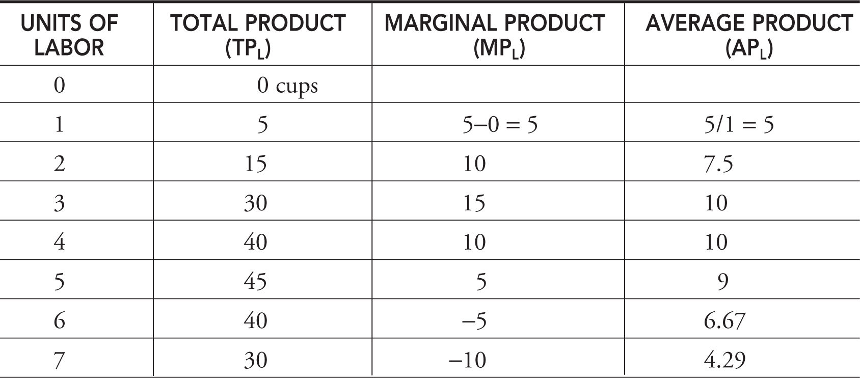
As Molly employs more workers to the fixed plant capacity (the table on the corner), total product increases, eventually peaks, and then begins to fall. This production function can be seen in Figure 8.1 .
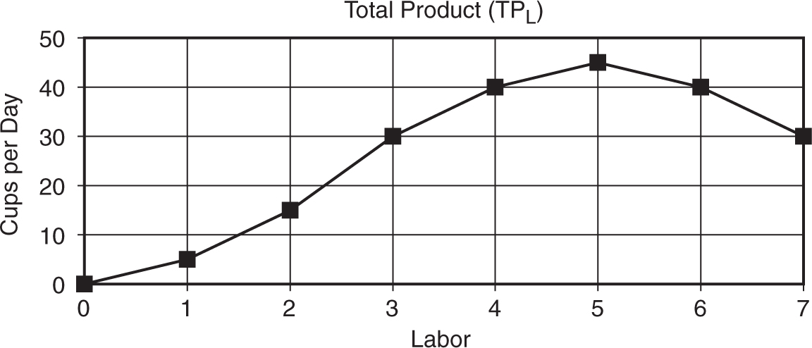
Figure 8.1
Law of Diminishing Marginal Returns
Imagine what happens to the lemonade stand as Molly adds more and more workers. At first, tasks are divided. (For example, Josh squeezes the lemons; Molly adds the sugar; Kelli stirs.) Specialization occurs. The marginal productivity of successive workers is rising in the early stage of production, but at some point, adding more workers increases the total product by a lesser amount. Maybe the fourth worker is pouring the lemonade and stocking while the fifth is taking money and making change. Beyond the fifth worker, the table is too crowded with employees, cups are spilled, product is wasted, and total production actually falls. The marginal contribution of these workers is negative. This illustrates one of the most important production concepts in the short run, the law of diminishing marginal returns , which states that as successive units of a variable resource are added to a fixed resource, beyond some point the marginal product falls .
“An important principle to know and understand.”
—AP Teacher

• Increasing marginal returns: MPL increases as L increases.
• Diminishing marginal returns: MPL decreases as L increases.
• Negative marginal returns: MPL becomes negative as L increases.
Graphically Speaking
Marginal product is the incremental change in total product as one more unit of labor is added. Marginal product is the geometric slope of total product. In Figure 8.1 , the total product curve is initially getting steeper as more labor is added. This is seen in Figure 8.2 as increasing marginal product. From the third to the fifth worker, the slope of total product is still positive, but it is becoming less steep. In Figure 8.2 marginal product from workers 3 to 5 is still positive but is falling. Beyond the fifth worker, total product is falling and thus has a negative slope. This turn of events is seen below when marginal product becomes negative.
Average product, also plotted below, initially rises, reaches a peak, and then begins to fall. So long as the marginal (next) worker adds production that is above the current average, they are pulling the average up. This is why we see APL rising so long as MPL is above APL . If the marginal worker adds production that is below the current average, the worker pulls the average down. Thus, when MPL is below APL , you see that APL is falling. Logically then, MPL intersects APL at the peak of APL . Average product cannot be negative.
• If MPL > APL : APL is rising.
• If MPL < APL : APL is falling.
• If MPL = APL : APL is at the peak.
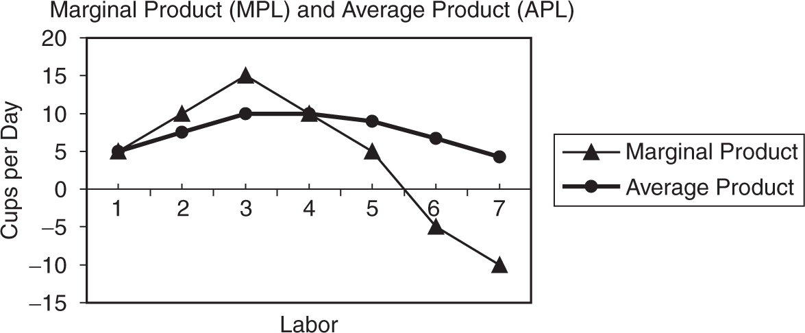
Figure 8.2
Short-Run Costs
It is important to note that we have discussed production theory without including the nagging necessity of paying for our hired inputs. For every employed input, fixed or variable, a cost is incurred.
Total Costs
In the short run, there is at least one input that is fixed and so these costs are also fixed. All inputs that are variable incur variable costs.
1. Total fixed costs (TFC) are those costs that do not vary with changes in short-run output. They must be paid even when output is zero. These include rent on building or equipment, insurance, or licenses.
2. Total variable costs (TVC) are those costs that change with the level of output. If output is zero, so are total variable costs. They include payment for materials, fuel, power, transportation services, most labor, and similar costs.
3. Total cost (TC) is the sum of total fixed and total variable costs at each level of output:
TC = TVC + TFC
Table 8.3
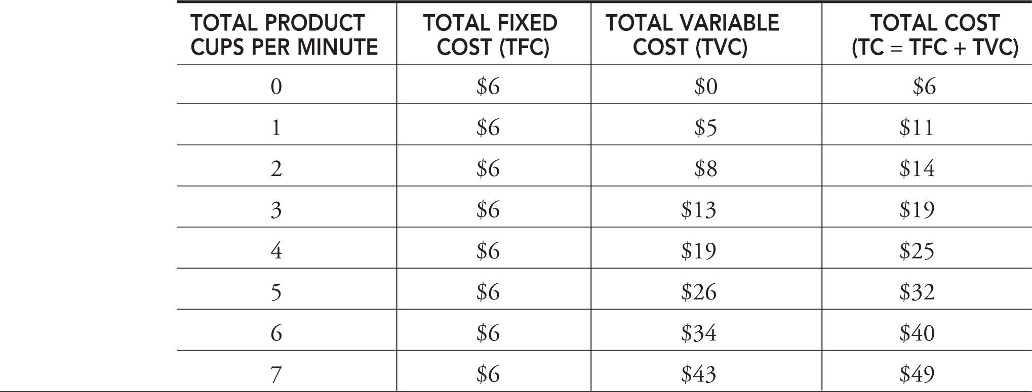
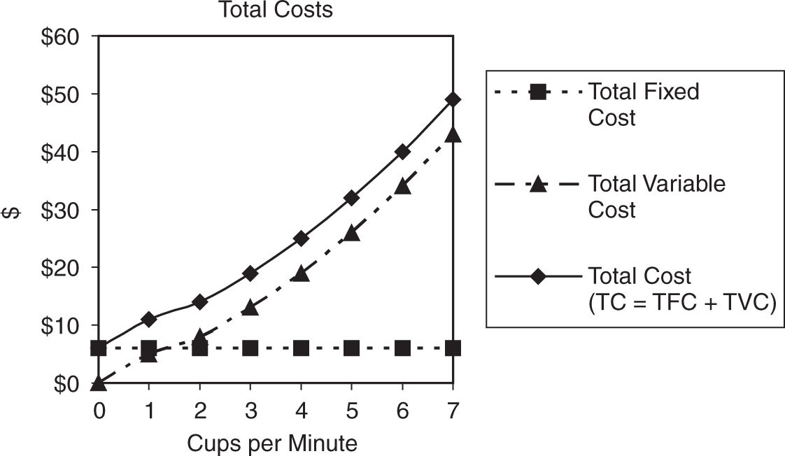
Figure 8.3
Table 8.3 summarizes Molly’s costs of producing cups of lemonade per minute. Her total fixed costs are assumed to be $6 per minute, and total variable costs increase as production increases.
Figure 8.3 illustrates the three total cost functions. Total fixed cost is a constant at all levels of output. Total variable cost quickly rises at first, briefly slows, and then proceeds to increase at an increasing rate. Total cost is simply the sum of TFC and TVC at every level of output, and so it lies parallel to TVC. Thus, the vertical distance between TC and TVC is equal to TFC.
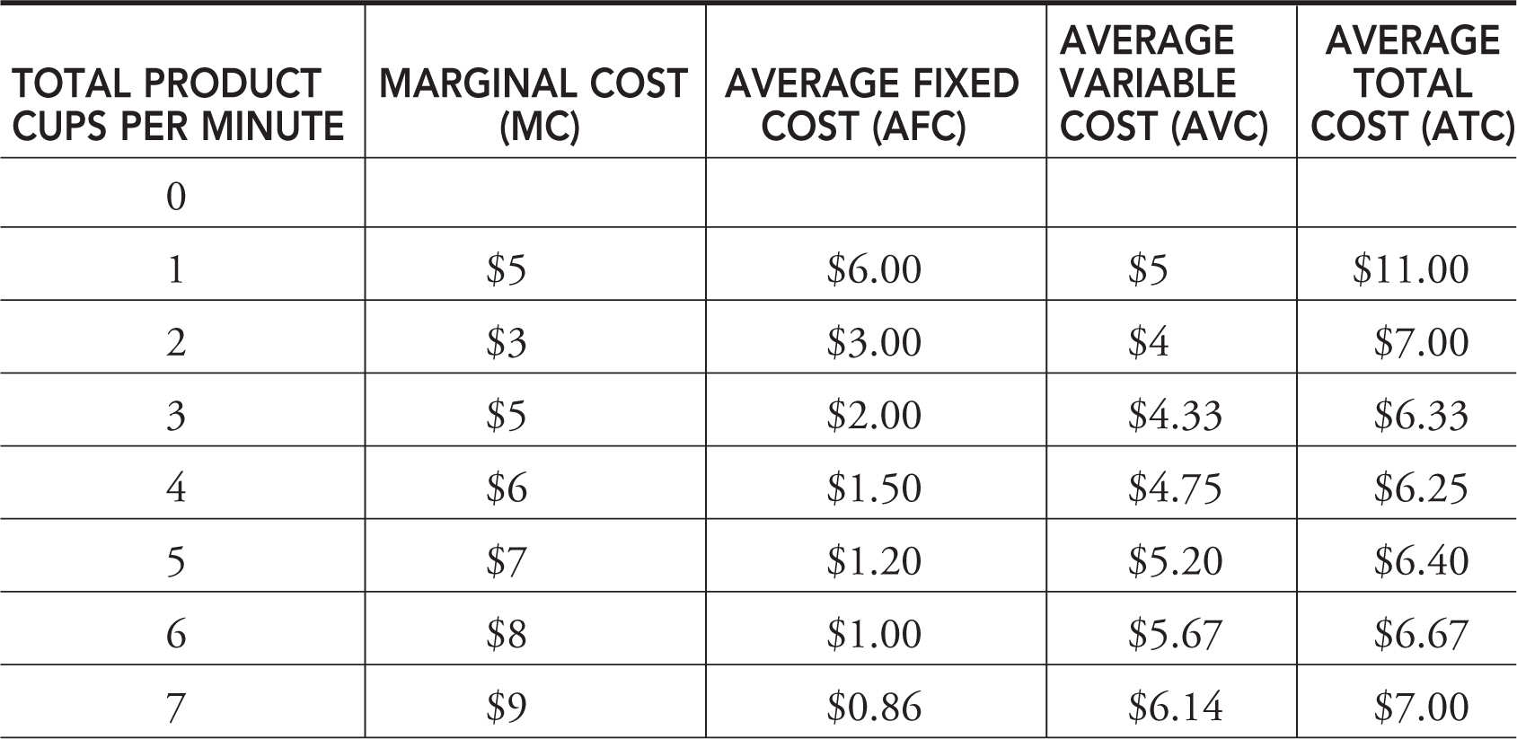
Table 8.4
Marginal and Average Costs
Similar to our discussion of production, we can derive marginal and per unit measures of cost from the total cost functions. These are in Table 8.4 .
1. Marginal cost is the additional cost of producing one more unit of output MC = ΔTC/ΔQ . Since TVC are the only costs that change with the level of output, marginal cost is also calculated as MC = ΔTVC/ΔQ . If quantity is changing one unit at a time, MC = ΔTC = ΔTVC.
2. Average fixed cost (AFC) is total fixed cost divided by output: AFC = TFC/Q . It continuously falls as output rises.
3. Average variable cost (AVC) is total variable cost divided by output: AVC = TVC/Q .
4. Average total cost (ATC) is total cost divided by output ATC = TC/Q . Note that ATC = AFC + AVC.
Graphically Speaking
If marginal product is the slope of total product, it should be no surprise that marginal cost is the slope of total cost, or total variable cost. We can see that marginal cost initially falls due to specialization but soon begins to rise as more output is produced. This is the law of increasing costs and is a direct result of the law of diminishing marginal returns to production. Both being U-shaped curves, average variable and average total costs initially fall, hit a minimum point, and begin to rise. Average total cost is vertically above AVC by the amount of AFC. Figure 8.4 illustrates this.
“It’s all about the graphs . . . if you can see it, you got it.”
—Cleo, AP Student
Marginal cost and average variable and average total cost are related in much the same way as marginal product is related to average product of labor. When the marginal cost of producing another cup of lemonade exceeds the current average cost, the average is rising. When the marginal cost of producing another cup of lemonade falls below the current average cost, the average is falling. Therefore, marginal cost equals average total cost at the minimum of ATC and equals average variable cost at the minimum of AVC.
When drawing a graph similar to the one in Figure 8.4 , it is important that you show an upward-sloping MC curve intersecting AVC and ATC at the minimum of those U-shaped curves. You can lose free-response points for sloppy graphs that show MC intersecting AVC and ATC at a point that is not clearly the minimum point, or bottom of the U-shaped curves.
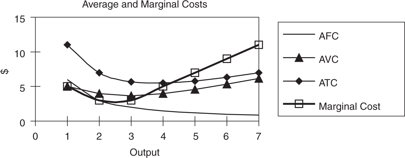
Figure 8.4
Here are three easy steps to drawing a clean graph that avoids any lost graphing points:
• Draw the upward-sloping curve and label it MC.
• Draw a downward-sloping curve that stops at the MC curve. Lift your pen from the paper. Trust me, if you try to draw the U in one smooth movement, you are more likely to lose this point.
• Beginning at the point where your downward sloping curve intersects MC, draw an upward sloping curve to complete the U-shaped ATC curve. You can repeat these steps to draw the AVC curve that lies below the ATC curve.
The mathematical relationship between total costs and per-unit (or average) costs is rather straightforward: divide the total dollars of cost by the output produced, and you get average dollars spent on a unit of output. These relationships can also be seen in a graph similar to the one in Figure 8.4 , and recent free-response questions have tested these relationships by asking students to use an average-cost graph like the one in Figure 8.5 to identify a total cost concept.
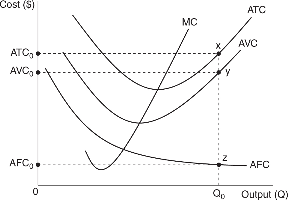
Figure 8.5
Suppose the firm is producing Q0 units of output. How can we determine total cost (TC0 ), total variable cost (TVC0 ), and total fixed cost (TFC0 ) from the information in Figure 8.5 ? Let’s take the relationship between ATC and TC as an example. Remember that average total cost is computed as
ATC0 = TC0 /Q0
so TC0 = ATC0 × Q0 . In Figure 8.5 , TC0 is the area of a rectangle with a width of Q0 units and a height of ATC0 . Using the notation in the graph, this area would be identified by the area 0ATC0 x Q0 . In a similar way, the TVC0would be identified by the area 0AVC 0 y Q0 , and TFC0 by the area 0AFC0 z Q0 .
If you know the relationships between total and per-unit costs, and you can identify the area in a graph like Figure 8.5 , you are prepared to earn some valuable free-response points.
Bridge over (Troubling) Economic Waters
Many students think that production and cost concepts are two sets of theoretical topics. This separation creates the impression that “there’s twice as much to remember.” These students are surprised to find out that production and cost are closely connected.
Think about it from Molly’s point of view. If the next worker employed has a high marginal product, then the marginal cost of producing that increased product must be quite low. When things are going well with production, they must be going well with cost. Try to see the concepts of production and cost not as two isolated bodies of theory but as two related sets of concepts that just need to be bridged. Let us try to build this bridge with a little algebra.
Marginal Product and Marginal Cost
MC = ΔTVC/ΔQ , and since the only variable input is labor being paid a fixed wage w ,
MC = w ΔL/ ΔQ which can be modified as,
MC = w/ (ΔQ/ ΔL) = w /MPL . MC and MPL are inverses of each other!
• As MPL is falling (diminishing marginal returns), MC is rising.
• As MPL is rising (increasing marginal returns), MC is falling.
• When MPL is highest, MC is lowest.
Average Product and Average Variable Cost
AVC = TVC/Q and with the only variable input being labor paid a fixed wage w ,
AVC = w L/Q which can be modified as,
AVC = w/ (Q/ L) = w /APL . AVC and APL are inverses of each other!
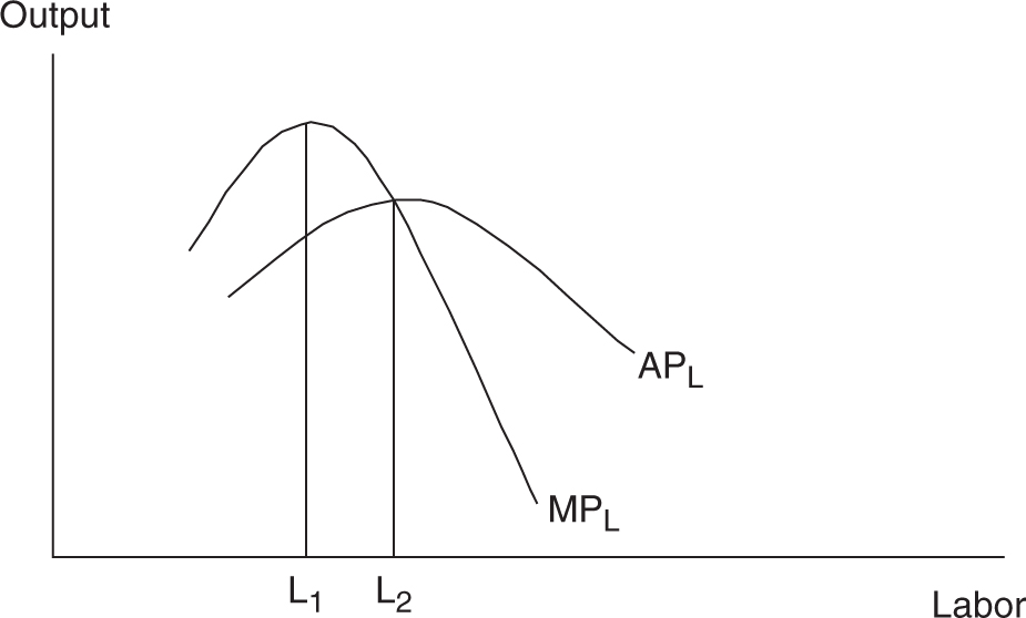
Figure 8.6
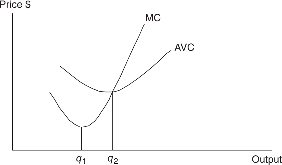
Figure 8.7
• As APL is falling, AVC is rising.
• As APL is rising, AVC is falling.
• When APL is highest, AVC is lowest.
If we put smoother versions of our production and cost figures together, we can see these relationships in Figures 8.6 and 8.7 .
“Make sure you know the definition for the Law of Diminishing Marginal Returns. It could appear in lots of different questions.”
—Cassie, AP Student
Long-Run Costs
Since all inputs are variable in the long run, discussion of production levels isn’t so much about output per hour or day; it’s more a question of plant size or capacity. In the short run, the firm asks, “With our current plant size, how much must we produce today?” The long run is long enough to adjust the plant capacity so the issue is really one of scale. The firm might ask itself, “At what scale do we want to operate?”
Long-Run Average Cost
I like to think of the firm’s short-run average costs as a snapshot of the firm’s ability to produce efficiently at the fixed plant size . Over time, the firm may grow and expand the plant size and begin to produce efficiently, but at the larger fixed plant size, giving us another snapshot. This process repeats itself as the firm expands or contracts and each time we receive another short-run snapshot of average cost. If we could put these short-run snapshots together into a kind of motion picture, we would see a more continuous long-run home movie of the firm’s average costs. The example and Figure 8.8 illustrate the connection between short- and long-run average costs.
“Make sure you can differentiate between long-run and short-run curves.”
—Kristy, AP Student
Example:
• In year one, Molly’s firm operates at a “small” scale, producing on SRAC1 .
• In year two, Molly could expand and operate at a “medium” scale, producing on SRAC2 , but only if she can sell more than 100 gallons of lemonade. At quantities below 100, SRAC1 < SRAC2 , so expansion would not be wise.
• In year three, Molly might expand to operate at a “large” scale and move to SRAC3 , but only if she can sell more than 250 gallons.
• Beyond the “large” scale exists a “grande” scale, but very quickly SRAC4 > SRAC3 and so this plant capacity actually begins to incur rising per unit costs.
Each of these four short-run snapshots of average costs can be smoothed out into the home movie long-run average cost curve, which is composed of sections of each short-run average cost curve at each of the four plant sizes that Molly might choose for her firm. In Figure 8.8 , the long-run average cost curve would lie along the segments a→b→c→d→e.
Economies of Scale
Construction of a smoother version of Figure 8.8 allows us to see more easily some important stages of the long-run average cost curves (Figure 8.9 ).
1. Economies of scale are advantages of increased plant size and are seen on the downward part of the LRAC curve. LRAC falls as plant size rises.
a. Labor and managerial specialization is one reason for this.
b. Ability to purchase and use more efficient capital goods also can explain economies of scale.
2. Constant returns to scale can occur when LRAC is constant over a variety of plant sizes.
3. Diseconomies of scale are illustrated by the rising part of the LRAC curve and can occur if a firm becomes too large.
a. Some reasons for this include distant management, worker alienation, and problems with communication and coordination.
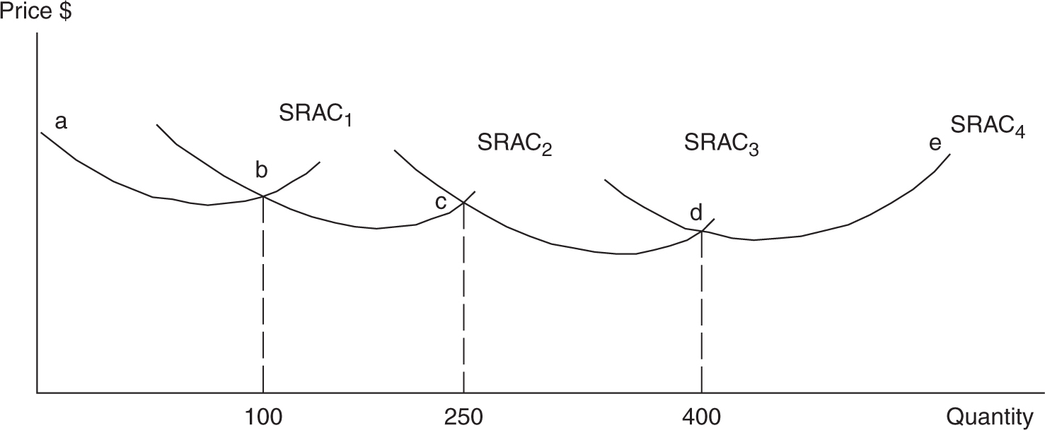
Figure 8.8
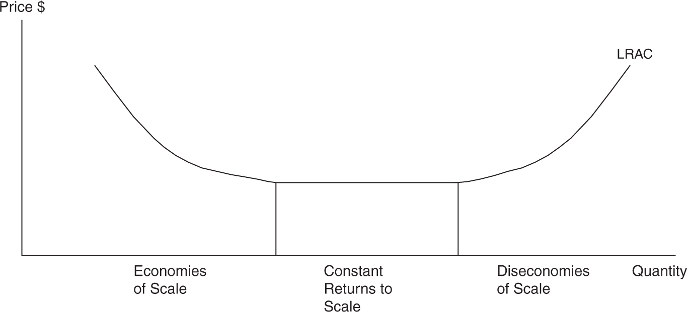
Figure 8.9
![]() Review Questions
Review Questions
1 . Which of the following is most likely an example of production inputs that can be adjusted in the long run, but not in the short run?
(A) Amount of wood used to make a desk.
(B) Number of pickles put on a sandwich.
(C) The size of a McDonald’s kitchen.
(D) Number of teacher’s assistants in local high schools.
(E) The amount of electricity consumed by a manufacturing plant.
2 . The Law of Diminishing Marginal Returns is responsible for
(A) AVC that first rises, but eventually falls, as output increases.
(B) AFC that first rises, but eventually falls, as output increases.
(C) MP that first falls, but eventually rises, as output increases.
(D) MC that first falls, but eventually rises, as output increases.
(E) ATC that first rises, but eventually falls, as output increases.
3 . Which of the following cost and production relationships is inaccurately stated?
(A) AFC = AVC – ATC
(B) MC = ΔTVC/ΔQ
(C) TVC = TC – TFC
(D) APL = TPL /L
(E) MC = w /MPL
4 . If the per unit price of labor, a variable resource, increases, it causes which of the following?
(A) An upward shift in AFC.
(B) An upward shift in MPL .
(C) A downward shift in ATC.
(D) An upward shift in MC.
(E) A downward shift in AFC.
Use the following figure to respond to questions 5 to 6.
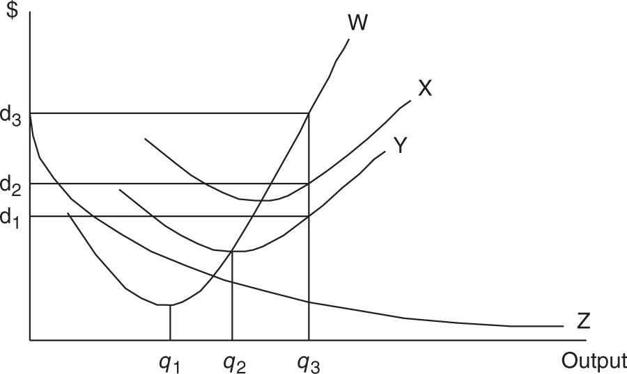
5 . The curves labeled W, X, Y, Z refer to which respective cost functions?
(A) MC, AVC, ATC, and AFC.
(B) MC, TC, TVC, and AFC.
(C) MC, ATC, AVC, and AFC.
(D) MC, ATC, AVC, and TFC.
(E) ATC, AVC, AFC, and MC.
6 . At the q 3 level of output,
(A) AFC = $d2 – $d1 .
(B) MC = $d2 .
(C) TVC = $d2 .
(D) ATC = $d3 .
(E) AFC = $d3 – $d2 .
![]() Answers and Explanations
Answers and Explanations
1 . C —The short run is a period of time too short to increase the plant size. All other choices involve decisions that could increase production almost immediately, with no change in the size of the facility. Increasing the size of a McDonald’s kitchen takes quite some time and represents an increase in the total capacity of the kitchen to produce.
2 . D —The law of diminishing marginal returns says that MPL eventually falls as you add more labor to a fixed plant. This question tests you on the important connection between production and cost. Remember that we derived this “bridge” and found that MC = w/ MPL . So when MPL is initially rising, MC is falling. Eventually when MPL is falling, MC is rising. Choices A, B, and E are just flat wrong. All three average costs begin by falling. AFC continues to fall, but AVC and ATC eventually rise.
3 . A —AFC plus AVC equals ATC. If you do the subtraction, AFC = ATC – AVC, making choice A the only incorrect statement. If you have studied your production and cost relationships, you recognize that choices B, C, D, and E are all stated correctly.
4 . D —When labor is more expensive, the MC of producing the good increases, so the MC curve shifts upward. The price of a variable input has increased, so easily rule out any reference to fixed costs. If anything, a higher wage shifts MPL downward.
5 . C —You must be familiar with the graphical representation of marginal and average cost functions.
6 . A —The vertical distance between ATC and AVC is AFC at any level of output.
![]() Rapid Review
Rapid Review
The firm: An organization that employs factors of production to produce a good or service that it hopes to profitably sell.
Accounting profit: The difference between total revenue and total explicit costs.
Economic profit: The difference between total revenue and total explicit and implicit costs.
Explicit costs: Direct, purchased, out-of-pocket costs paid to resource suppliers outside the firm. Also referred to as accounting costs .
Implicit costs: Indirect, non-purchased, or opportunity costs of resources provided by the entrepreneur. Also called economic costs .
Short run: A period of time too short to change the size of the plant, but many other, more variable resources can be adjusted to meet demand.
Long run: A period of time long enough to alter the plant size. New firms can enter the industry and existing firms can liquidate and exit.
Production function: The mechanism for combining production resources, with existing technology, into finished goods and services. Inputs are turned into outputs.
Fixed inputs: Production inputs that cannot be changed in the short run. Usually this is the plant size or capital.
Variable inputs: Production inputs that the firm can adjust in the short run to meet changes in demand for their output. Often this is labor and/or raw materials.
Total Product of Labor (TP L ): The total quantity, or total output, of a good produced at each quantity of labor employed.
Marginal Product of Labor (MP L ): The change in total product resulting from a change in the labor input. MPL = ΔTPL /ΔL, or the slope of total product.
Average Product of Labor (AP L ): Total product divided by labor employed: APL = TPL /L.
Law of diminishing marginal returns: As successive units of a variable resource are added to a fixed resource, beyond some point the marginal product declines.
Total fixed costs (TFC): Costs that do not vary with changes in short-run output. They must be paid even when output is zero.
Total variable costs (TVC): Costs that change with the level of output. If output is zero, so are total variable costs.
Total cost (TC): The sum of total fixed and total variable costs at each level of output: TC = TVC + TFC.
Marginal cost (MC): The additional cost of producing one more unit of output. MC = ΔTC/ΔQ = ΔTVC/ΔQ or the slope of total cost and total variable cost.
Average fixed cost (AFC): Total fixed cost divided by output: AFC = TFC/Q .
Average variable cost (AVC): Total variable cost divided by output: AVC = TVC/Q .
Average total cost (ATC): Total cost divided by output. ATC = TC/Q = AFC + AVC.
Relationship between MP L and MC: If labor is the variable input being paid a fixed wage (w ), MC and MP L are inverses of each other. MC = w/ (ΔQ/ ΔL) = w /MPL .
Relationship between AP L and AVC: In the simplified case where labor is the variable input being paid a fixed wage (w ), AVC and APL are inverses of each other. AVC = w/ (Q /L) = w /APL .
Economies of scale: The downward part of the LRAC curve where LRAC falls as plant size increases. This is the result of specialization, lower cost of inputs, or other efficiencies from larger scale.
Constant returns to scale: Occurs when LRAC is constant over a variety of plant sizes.
Diseconomies of scale: The upward part of the LRAC curve where LRAC rises as plant size increases. This is usually the result of the increased difficulty of managing larger firms, which results in lost efficiency and rising per unit costs.