1,001 Calculus Practice Problems
Part II
The Answers
In this part …
Here you get answers and explanations for all 1,001 problems. As you read the solutions, you may realize that you need a little more help. Lucky for you, the For Dummies series (published by Wiley) offers several excellent resources. I recommend checking out the following titles, depending on your needs:
· Calculus For Dummies, Calculus Workbook For Dummies, and Calculus Essentials For Dummies, all by Mark Ryan
· Pre-Calculus For Dummies, by Yang Kuang and Elleyne Kase, and Pre-Calculus Workbook For Dummies, by Yang Kuang and Michelle Rose Gilman
· Trigonometry For Dummies and Trigonometry Workbook For Dummies, by Mary Jane Sterling
When you're ready to step up to more advanced calculus courses, you'll find the help you need in Calculus II For Dummies, by Mark Zegarelli.
Visit www.dummies.com for more information.
Chapter 16
Answers and Explanations
Here are the answer explanations for all 1,001 practice problems.
1. ![]()
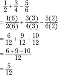
Get a common denominator of 12 and then perform the arithmetic in the numerator:
2. ![]()
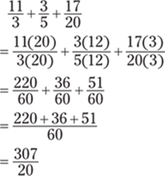
Get a common denominator of 60 and then perform the arithmetic in the numerator:
3. 11
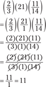
Write each factor as a fraction and then multiply across the numerator and denominator (cancel common factors as well!):
4. ![]()
Recall that to divide by a fraction, you multiply by its reciprocal:  . After rewriting the fraction, cancel common factors before multiplying:

5. 
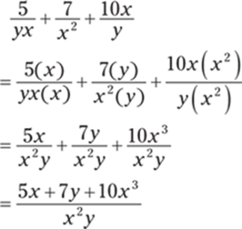
To add the fractions, you need a common denominator. The least common multiple of the denominators is x2y, so multiply each fraction accordingly to get this denominator for each term. Then write the answer as a single fraction:
6. ![]()
You need a common denominator so you can subtract the fractions. The least common multiple of the denominators is (x – 1)(x + 1) = x2 – 1, so multiply each fraction accordingly to get this denominator. Then perform the arithmetic in the numerator:
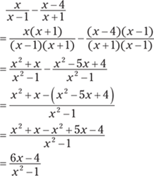
7. ![]()
Begin by factoring the expressions completely. Cancel any common factors and then simplify to get the answer:
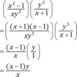
8. 
Recall that to divide by a fraction, you multiply by its reciprocal:  . After rewriting the fraction, factor and cancel the common factors:
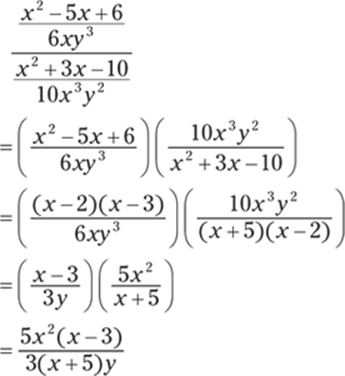
9. ![]()
Write each factor using positive exponents and then simplify. To start, notice that ![]() in the denominator becomes
in the denominator becomes ![]() when it moves to the numerator:
when it moves to the numerator:
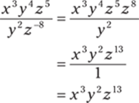
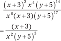
10. 
To simplify, cancel the common factors:
11. ![]()
Because the entire expression is being raised to the power of zero, the answer is 1:

There's no point in simplifying the expression inside the parentheses.
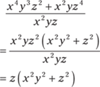
12. ![]()
Begin by factoring the numerator and then cancel the common factors:
13. 
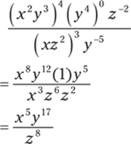
For this problem, you need to know the properties of exponents. The important properties to recall here are ![]() ,
, ![]() ,
, ![]() ,
, ![]() ,
, ![]() , and
, and ![]() .
.
Write all factors using positive exponents and then use the properties of exponents to simplify the expression:
14. ![]()
Factor the number underneath the radical and then rewrite the radical using ![]() to simplify:
to simplify:

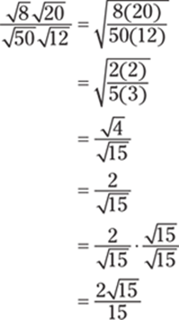
15. ![]()
Start by rewriting the expression so it has only one square root sign. Then reduce the fraction and use properties of radicals to simplify:
16. ![]()
Begin by writing the expression using a single square root sign. Then combine like bases and simplify:
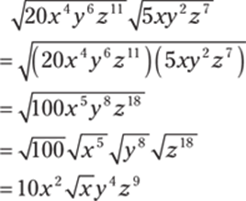
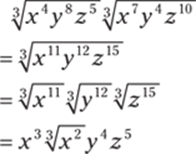
17. ![]()
Begin by writing the expression using a single cube root sign. Combine the factors with like bases and then simplify:
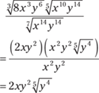
18. ![]()
Simplify each root individually and then use properties of exponents to simplify further:
19. ![]()
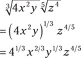
Recall that ![]() . The expression becomes
. The expression becomes

20. ![]()
Recall that ![]() . Therefore, the expression becomes
. Therefore, the expression becomes
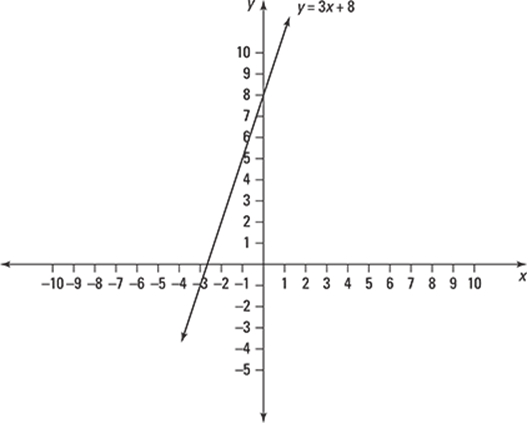
21. y = 3x + 8
Recall that a function is one-to-one if it satisfies the requirement that if x1 ≠ x2, then f (x1) ≠ f (x2); that is, no two x coordinates have the same y value. If you consider the graph of such a function, no horizontal line would cross the graph in more than one place.
Of the given functions, only the linear function y = 3x + 8 passes the horizontal line test. This function is therefore one-to-one and has an inverse.
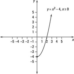
22. y = x2 – 4, x ≥ 0
When determining whether a function has an inverse, consider the domain of the given function. Some functions don't pass the horizontal line test — and therefore don't have an inverse — unless the domain is restricted. The function y = x2 – 4 doesn't pass the horizontal line test; however, if you restrict the domain to x ≥ 0, then y = x2 – 4 does pass the horizontal line test (and therefore has an inverse), because you're getting only the right half of the parabola.
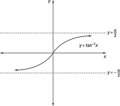
23. y = tan−1 x
Of the given functions, only the function y = tan−1 x passes the horizontal line test. Therefore, this function is one-to-one and has an inverse.
24. ![]()
First replace f (x) with y:

Then replace y with x and each x with y. After making the replacements, solve for y to find the inverse:
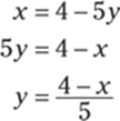
Therefore, the inverse of f (x) = 4 – 5x is
![]()
25. ![]()
First replace f (x) with y:

Then replace y with x and each x with y. After making the replacements, solve for y to find the inverse. You need to complete the square so you can isolate y. (To complete the square, consider the quadratic expression on the right side of the equal sign; take one-half of the coefficient of the term involving y, square it, and add that value to both sides of the equation.) Then factor the right side and use square roots to solve for y:
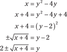
Notice that for the domain of the inverse to match the range of f (x), you have to keep the positive root. Therefore, the inverse of f (x) = x2 – 4x, where x ≥ 2, is
![]()
26. ![]() ,
, ![]()
First replace f (x) with y:

Then replace y with x and each x with y. After making the replacements, solve for y to find the inverse:
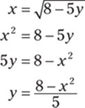
Therefore, the inverse of ![]() is
is
![]()
The domain of the inverse is x ≥ 0 because the range of f (x) is y ≥ 0 and the domain of ![]() is equal to the range of f (x).
is equal to the range of f (x).
27. ![]()
First replace f (x) with y:

Then replace y with x and each x with y. After making the replacements, solve for y to find the inverse:
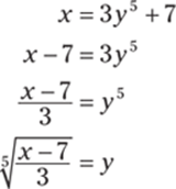
Therefore, the inverse of f (x) = 3x5 + 7 is
![]()
28. 
First replace f (x) with y:
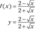
Then replace y with x and each x with y. After making the replacements, solve for y to find the inverse:
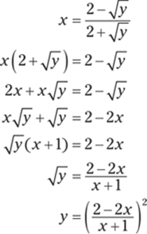
Note that the range of  is (–1, 1], so the domain of the inverse function is (–1, 1]. Therefore, the inverse of
  is
is

29. ![]()
First replace f (x) with y:

Then replace y with x and each x with y. After making the replacements, solve for y to find the inverse:
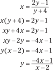
Therefore, the inverse of ![]() is
is
![]()
30. {(1, 0), (4, 3), (–6, 5)}
If the point (a, b) is on the graph of a one-to-one function, the point (b, a) is on the graph of the inverse function. Therefore, just switch the x and y coordinates to get that the set of points {(1, 0), (4, 3), (–6, 5)} belongs to the graph of f −1(x).
31. domain: (–1, 2); range: [–2, 4)
For a one-to-one function (which by definition has an inverse), the domain of f (x) becomes the range of f −1(x), and the range of f (x) becomes the domain of f −1(x). Therefore, f −1(x) has domain (–1, 2) and range [–2, 4).
32. g −1(x) = f −1(x) – c
Replacing x with (x + c) shifts the graph c units to the left, assuming that c > 0. If the point (a, b) belongs to the graph of f (x), then the point (a – c, b) belongs to the graph of f (x + c).
Now consider the inverse. The point (b, a) belongs to the graph of f −1(x), so the point (b, a – c) belongs to the graph of g −1(x). Therefore, g −1(x) is the graph of f −1(x) shifted down c units so that g −1(x) = f −1(x) – c.
The same argument applies if c < 0.
33. x = 2
Put all terms involving x on one side of the equation and all constants on the other side, combining all like terms. Finally, divide by the coefficient of x to get the solution:

34. x = –4
Distribute to remove the parentheses. Then put all terms involving x on one side of the equation and all constants on the other side, combining all like terms. Finally, divide by the coefficient of x to get the solution:
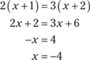
35. ![]()
Distribute to remove the parentheses. Then put all terms involving x on one side of the equation and all constants on the other side, combining all like terms. Finally, divide by the coefficient of x to get the solution:
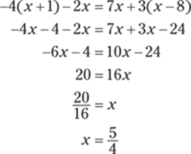
36. ![]()
Put all terms involving x on one side of the equation and all constants on the other side, combining all like terms. Finally, divide by the coefficient of x (that is, multiply both sides by the reciprocal of the coefficient) to get the solution:
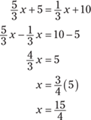
37. 
Distribute to remove the parentheses. Then put all terms involving x on one side of the equation and all constants on the other side, combining all like terms. Finally, divide by the coefficient of x to get the solution:
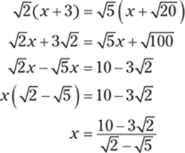
38. x = –3, 7
This quadratic factors without too much trouble using trial and error:

Setting each factor equal to zero gives you x – 7 = 0 so that x = 7 is a solution and x + 3 = 0 so that x = –3 is a solution.
39. ![]()
Complete the square to solve the quadratic equation. (To complete the square, consider the quadratic expression on the left side of the equal sign; take one-half of the coefficient of the term involving x, square it, and add that value to both sides of the equation.) Then factor the left side and use square roots to solve for x:
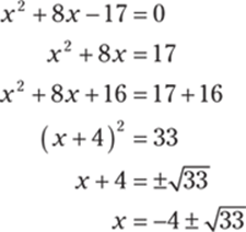
40. ![]()
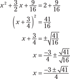
Complete the square to solve the quadratic equation. Begin by moving the constant to the right side of the equal sign and then dividing both sides of the equation by 2:
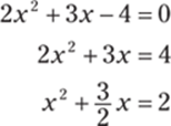
Next, consider the quadratic expression on the left side of the equal sign; take one-half of the coefficient of the term involving x, square it, and add that value to both sides of the equation. Then factor the left side and use square roots to solve for x:
41. ![]()
Factoring by trial and error gives you

Setting each factor equal to zero gives you 2x – 1 = 0 so that ![]() is a solution and 3x + 4 = 0 so that
is a solution and 3x + 4 = 0 so that ![]() is a solution.
is a solution.
42. ![]()
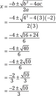
The equation 3x2 + 4x – 2 = 0 doesn't factor nicely, so use the quadratic equation to solve for x. Here, a = 3, b = 4, and c = –2:
43. ![]()
The equation x10 + 7x5 + 10 = 0 isn't quadratic, but by using a substitution, you can produce a quadratic equation:

Now use the substitution y = x5 to form a quadratic equation that you can easily factor:

From y + 2 = 0, you have the solution y = –2, and from y + 5 = 0, you have the solution y = –5.
Now replace y using the original substitution and solve for x to get the final answer: x5 = –2 gives you ![]() , and x5= –5 gives you
, and x5= –5 gives you ![]() .
.
44. x = 0, ![]() , 1
, 1
Begin by factoring out the greatest common factor, x2. Then factor the remaining quadratic expression:
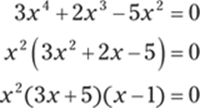
Next, set each factor equal to zero and solve for x: x2 = 0 has the solution x = 0, 3x + 5 = 0 has the solution ![]() , and x – 1 = 0 has the solution x = 1.
, and x – 1 = 0 has the solution x = 1.
45. no real solutions
Factoring this polynomial by trial and error gives you the following:

Setting the first factor equal to zero gives you x4 + 5 = 0 so that x4 = –5, which has no real solutions. Setting the second factor equal to zero gives you x4 + 7 = 0 so that x4 = –7, which also has no real solutions.
46. x = –1, 1
Factor the polynomial repeatedly to get the following:
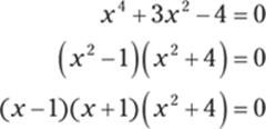
Now set each factor equal to zero and solve for x. Setting the first factor equal to zero gives you x – 1 = 0 so that x = 1. The second factor gives you x + 1 = 0 so that x = –1. And the last factor gives you x2 + 4 = 0 so that x2 = –4, which has no real solutions.
47. x = –3, 3
Factor the polynomial repeatedly to get the following:
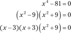
Now set each factor equal to zero and solve for x. Setting the first factor equal to zero gives you x – 3 = 0 so that x = 3. Setting the second factor equal to zero gives you x + 3 = 0 so that x = –3. The last factor gives you x2 + 9 = 0, or x2 = –9, which has no real solutions.
48. x = 1, ![]()
To solve an absolute value equation of the form ![]() , where b > 0, you must solve the two equations a = b and a = –b. So for the equation
, where b > 0, you must solve the two equations a = b and a = –b. So for the equation ![]() , you have to solve 5x – 7 = 2:
, you have to solve 5x – 7 = 2:

You also have to solve 5x – 7 = –2:

Therefore, the solutions are ![]() and x = 1.
and x = 1.
49. no real solutions
To solve an absolute value equation of the form ![]() , where b > 0, you must solve the two equations a = b and a = –b. However, in this case, you have
, where b > 0, you must solve the two equations a = b and a = –b. However, in this case, you have ![]() , which gives you
, which gives you ![]() . Because the absolute value of a number can't be negative, this equation has no solutions.
. Because the absolute value of a number can't be negative, this equation has no solutions.
50. x = –3, 9
To solve an absolute value equation of the form ![]() , where b > 0, you must solve the two equations a = b and a = –b. So for the equation
, where b > 0, you must solve the two equations a = b and a = –b. So for the equation ![]() , you must solve x2 – 6x = 27 and x2 – 6x = –27.
, you must solve x2 – 6x = 27 and x2 – 6x = –27.
To solve x2 – 6x = 27, set the equation equal to zero and factor using trial and error:

Setting each factor equal to zero gives you x – 9 = 0, which has the solution x = 9, and x + 3 = 0, which has the solution x = –3.
Then set x2 – 6x = –27 equal to zero, giving you x2 – 6x + 27 = 0. This equation doesn't factor nicely, so use the quadratic equation, with a = 1, b = –6, and c = 27:
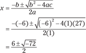
The number beneath the radical is negative, so this part of the absolute value has no real solutions.
Therefore, the only real solutions to ![]() are x = –3 and x = 9.
are x = –3 and x = 9.
51. x = –3, 2
To solve an absolute value equation of the form ![]() , you must solve the two equations a = b and a = –b. So for the equation
, you must solve the two equations a = b and a = –b. So for the equation ![]() , you have to solve 15x – 5 = 35 – 5x and 15x – 5 = –(35 – 5x).
, you have to solve 15x – 5 = 35 – 5x and 15x – 5 = –(35 – 5x).
For the first equation, you have

And for the second equation, you have
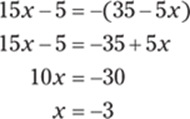
Therefore, the solutions are x = –3 and x = 2.
52. x = –1
To solve a rational equation of the form ![]() , you need to solve the equation p(x) = 0. Therefore, to solve
, you need to solve the equation p(x) = 0. Therefore, to solve ![]() , you simply set the numerator equal to zero and solve for x:
, you simply set the numerator equal to zero and solve for x:

53. x = ![]() ,
, ![]()
To solve the equation ![]() , first remove all fractions by multiplying both sides of the equation by the least common multiple of the denominators:
, first remove all fractions by multiplying both sides of the equation by the least common multiple of the denominators:
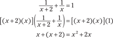
In this case, multiplying leaves you with a quadratic equation to solve:
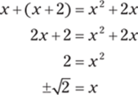
Check the solutions to see whether they're extraneous (incorrect) answers. In this case, you can verify that both ![]() and
and ![]() satisfy the original equation by substituting these values into
satisfy the original equation by substituting these values into ![]() and checking that you get 1 on the left side of the equation.
and checking that you get 1 on the left side of the equation.
54. –14
To solve an equation of the form ![]() , cross-multiply to produce the equation ad = bc:
, cross-multiply to produce the equation ad = bc:
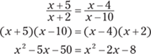
After cross-multiplying, you're left with a quadratic equation, which then reduces to a linear equation:

You can verify that –14 is a solution of the original rational equation by substituting x = –14 into the equation ![]() and checking that you get the same value on both sides of the equation.
and checking that you get the same value on both sides of the equation.
55. no real solutions
Begin by factoring all denominators. Then multiply each side of the equation by the least common multiple of the denominators to remove all fractions:

Then simplify:
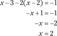
Because x = 2 makes the original equation undefined, there are no real solutions.
56. (–4, 8)
To solve the inequality x2 – 4x – 32 < 0, begin by solving the corresponding equation x2 – 4x – 32 = 0. Then pick a point from each interval (determined by the solutions) to test in the original inequality.
Factoring x2 – 4x – 32 = 0 gives you (x + 4)(x – 8) = 0. Setting the first factor equal to zero gives you x + 4 = 0, which has the solution x = –4, and setting the second factor equal to zero gives you x – 8 = 0, which has the solution x = 8.
Therefore, you need to pick a point from each of the intervals, (–∞, –4), (–4, 8), and (8, ∞), to test in the original inequality. Substitute each test number into the expression x2 – 4x – 32 to see whether the answer is less than or greater than zero.
Using x = –10 to check the interval (–∞, –4) gives you
![]()
which is not less than zero and so doesn't satisfy the inequality.
Using x = 0 to check the interval (–4, 8) gives you
![]()
which is less than zero and does satisfy the inequality.
Using x = 10 to check the interval (8, ∞) gives you
![]()
which is not less than zero and so doesn't satisfy the inequality.
Therefore, the solution set is the interval (–4, 8).
57. ![]()
To solve the inequality 2x4 + 2x3 ≥ 12x2, begin by setting one side equal to zero. Solve the corresponding equation and then pick a point from each interval (determined by the solutions) to test in the inequality.
So from 2x4 + 2x3 ≥ 12x2, you have 2x4 + 2x3 – 12x2 ≥ 0. Factoring the corresponding equation so you can solve for x gives you
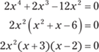
Set each factor equal to zero and solve for x, giving you the solutions x = 0,x = –3, and x = 2. These values are also solutions to the inequality.
Next, pick a test point from each of the intervals, (–∞, –3), (–3, 0), (0, 2), and (2, ∞), to see whether the answer is positive or negative. Using x = –10 to check the interval (–∞, –3) gives you

which is greater than zero.
Using x = –1 to check the interval (–3, 0) gives you

which is less than zero.
Using x = 1 to check the interval (0, 2) gives you

which is less than zero.
Finally, using x = 10 to check the interval (2, ∞) gives you

which is greater than zero.
Therefore, the solution set is ![]() .
.
Note that you could've divided the original inequality by 2 to simplify the initial inequality.
58. ![]()
To solve the rational inequality ![]() , first determine which values will make the numerator equal to zero and which values will make the denominator equal to zero. This helps you identify zeros (where the graph crosses the x-axis) and points where the function is not continuous.
, first determine which values will make the numerator equal to zero and which values will make the denominator equal to zero. This helps you identify zeros (where the graph crosses the x-axis) and points where the function is not continuous.
From the numerator, you have x + 1 = 0, which has the solution x = –1. You also have x – 2 = 0, which has the solution x = 2. From the denominator, you have x + 3 = 0, which has the solution x = –3. Take a point from each interval determined by these solutions and test it in the original inequality.
You need to test a point from each of the intervals, (–∞, –3), (–3, –1), (–1, 2), and (2, ∞). Pick a point from each interval and substitute into the expression ![]() to see whether you get a value less than or greater than zero.
to see whether you get a value less than or greater than zero.
Using x = –10 to test the interval (–∞, –3) gives you
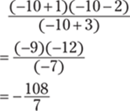
which is less than zero and so satisfies the inequality.
Using x = –2 to test the interval (–3, –1) gives you
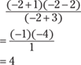
which is greater than zero and doesn't satisfy the inequality.
Using x = 0 to test the interval (–1, 2) gives you
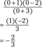
which is less than zero and so satisfies the inequality.
Using x = 3 to test the interval (2, ∞) gives you
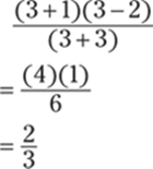
which is greater than zero and so doesn't satisfy the inequality.
Therefore, the solution set is the interval (–∞, –3) and (–1, 2).
59. ![]() (1, 3)
(1, 3)
Begin by putting the rational inequality into the form ![]() by putting all terms on one side of the inequality and then getting common denominators:
by putting all terms on one side of the inequality and then getting common denominators:
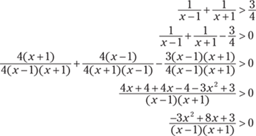
Next, set the numerator equal to zero and solve for x. Setting the numerator equal to zero gives you a quadratic equation that you can factor by trial and error:

The solutions are ![]() and x = 3.
and x = 3.
Also set each factor from the denominator equal to zero and solve for x. This gives you both (x – 1) = 0, which has the solution x = 1, and (x + 1) = 0, which has the solution x = –1.
Next, take a point from each of the intervals, (–∞, –1), ![]() ,
, ![]() , (1, 3), and (3, ∞), and test it in the expression
, (1, 3), and (3, ∞), and test it in the expression  to see whether the answeris positive or negative; or equivalently, you can use the expression
 ![]() .
.
Using x = –10 to test the interval (–∞, 1) gives you
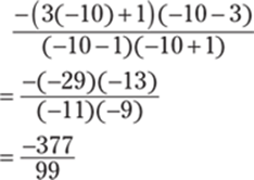
which is less than zero and so doesn't satisfy the inequality.
Using ![]() to test the interval
to test the interval ![]() gives you
gives you
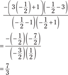
which is greater than zero and so satisfies the inequality.
Using x = 0 to test the interval ![]() gives you
gives you
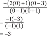
which is less than zero and so doesn't satisfy the inequality.
Using x = 2 to test the interval (1, 3) gives you
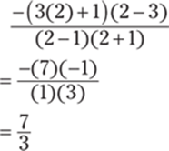
which is greater than zero and so satisfies the inequality.
And using x = 10 to test the interval (3, ∞) gives you
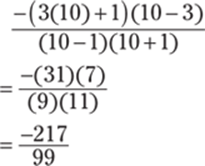
which is less than zero and so doesn't satisfy the inequality.
Therefore, the solution set is the intervals ![]() and (1, 3).
and (1, 3).
60. ![]()
To solve an absolute inequality of the form ![]() , where b > 0, solve the compound inequality –b < a < b. So for the inequality
, where b > 0, solve the compound inequality –b < a < b. So for the inequality ![]() , you have
, you have
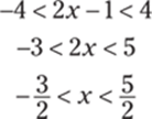
The solution set is ![]() .
.
61. (–∞, 1) ![]()
To solve an absolute value inequality of the form ![]() , where b > 0, you have to solve the corresponding inequalities a > b and a < –b. Therefore, for the inequality
, where b > 0, you have to solve the corresponding inequalities a > b and a < –b. Therefore, for the inequality ![]() , you have to solve 5x – 7 > 2 and 5x – 7 < –2. For the first inequality, you have
, you have to solve 5x – 7 > 2 and 5x – 7 < –2. For the first inequality, you have

And for the second inequality, you have

Therefore, the solution set is the intervals (–∞, 1) and ![]() .
.
62. ![]()
To solve an absolute inequality of the form ![]() , where b > 0, solve the compound inequality –b ≤ a ≤ b. For the inequality
, where b > 0, solve the compound inequality –b ≤ a ≤ b. For the inequality ![]() , you have
, you have
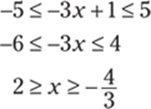
Therefore, the solution is the interval ![]() .
.
63. ![]()
The slope of a line that goes through the points (x1, y1) and (x2, y2) is given by ![]() . Therefore, the slope of the line that passes through (1, 2) and (5, 9) is
. Therefore, the slope of the line that passes through (1, 2) and (5, 9) is
![]()
64. y = 4x + 5
The graph of y = mx + b is a line with slope of m and a y-intercept at (0, b). Therefore, using m = 4 and b = 5 gives you the equation y = 4x + 5.
65. ![]()
The equation of a line that goes through the point (x1, y1) and has a slope of m is given by the point-slope formula: y – y1 = m(x – x1).
The slope of the line that goes through (–2, 3) and (4, 8) is
![]()
Now use the slope and the point (4, 8) in the point-slope formula:
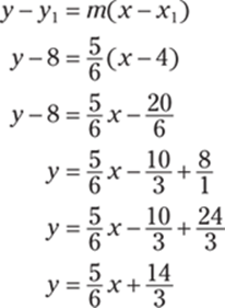
66. ![]()
The equation of a line that goes through the point (x1, y1) and has a slope of m is given by the point-slope formula: y – y1 = m(x – x1).
The two lines are parallel, so the slopes are the same. Therefore, the slope of the line you're trying to find is ![]() .
.
Using the slope and the point (1, 5) in the point-slope formula gives you
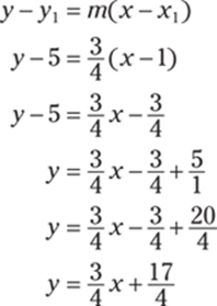
67. ![]()
The equation of a line that goes through the point (x1, y1) and has a slope of m is given by the point-slope formula: y – y1 = m(x – x1).
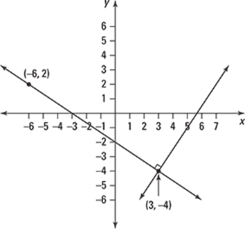
The slope of the line that goes through the points (–6, 2) and (3, –4) is
![]()
The slopes of perpendicular lines are opposite reciprocals of each other, so the slope of the line you want to find is ![]() (you flip the fraction and change the sign).
(you flip the fraction and change the sign).
Using the slope and the point (3, –4) in the point-slope formula gives you
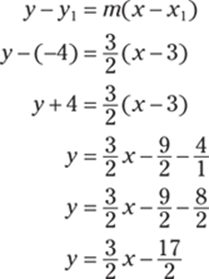
Here's what the perpendicular lines look like:
68. ![]()
Stretching the graph of ![]() vertically by a factor of 2 produces the equation
vertically by a factor of 2 produces the equation ![]() . To shift the graph of
. To shift the graph of ![]() to the right 3 units, replace x with (x – 3) to get
to the right 3 units, replace x with (x – 3) to get ![]() . Last, to move the graph of
. Last, to move the graph of ![]() up 4 units, add 4 to the right side to get
up 4 units, add 4 to the right side to get ![]() .
.
69. ![]()
The vertex form of a parabola is given by y = a(x – h)2 + k, with the vertex at the point (h, k). Using the vertex (–2, –4) gives you the following equation:

Now use the point (0, 2) to solve for a:
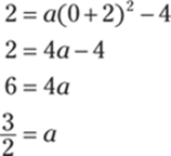
Therefore, the equation of the parabola is
![]()
70. y = –(x + 1)2 + 6
The vertex form of a parabola is given by y = a(x – h)2 + k, with the vertex at the point (h, k). Using the vertex (–1, 6), you have the following equation:

Now use the point (1, 2) to solve for a:
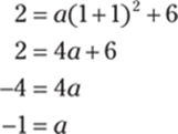
Therefore, the vertex form of the parabola is
![]()
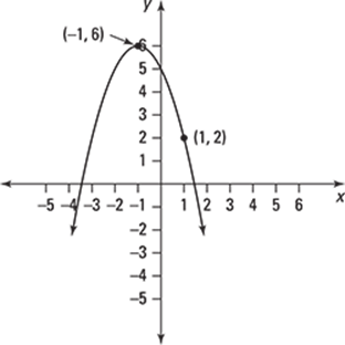
Here's the graph of y = –(x + 1)2 + 6:
71. y = 3(x – 5)2 + 2
To translate the parabola 6 units to the right, you replace x with the quantity (x – 6). And to translate the parabola 2 units down, you subtract 2 from the original expression for y:

Another option is simply to count and determine that the new vertex is at (5, 2); then use the vertex form y = a(x – h)2 + k, where the vertex is at the point (h, k).
72. y = e−2x – 5
To compress the graph of y = ex horizontally by a factor of 2, replace x with 2x to get y = e2x. To reflect the graph of y = e2x across the y-axis, replace x with –x to get y = e2(–x), or y = e−2x. Last, to shift the graph of y = e−2x down 5 units, subtract 5 from the right side of the equation to get y = e−2x – 5.
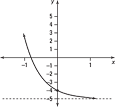
Here's the graph of y = e−2x – 5:
73. ![]()
To stretch the graph of ![]() horizontally by a factor of 5, replace x with
horizontally by a factor of 5, replace x with ![]() to get
to get ![]() . Next, to reflect the graph of
. Next, to reflect the graph of ![]() across the x-axis, multiply the right side of the equation
across the x-axis, multiply the right side of the equation ![]() by –1 to get
by –1 to get ![]() . Last, to shift the graph of
. Last, to shift the graph of ![]() up 3 units, add 3 to the right side of the equation to get
up 3 units, add 3 to the right side of the equation to get
![]()
74. ![]()
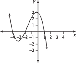
The polynomial has x intercepts at x = –4, x = –2, and x = 1, so you know that the polynomial has the factors (x + 4), (x + 2), and (x – 1). Therefore, you can write
![]()
Use the point (0, 3) to solve for a:
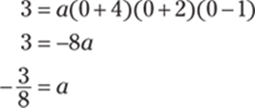
Now you can enter the value of a in the equation of the polynomial and simplify:
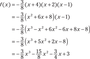
Here's the graph of ![]() :
:
75. ![]()
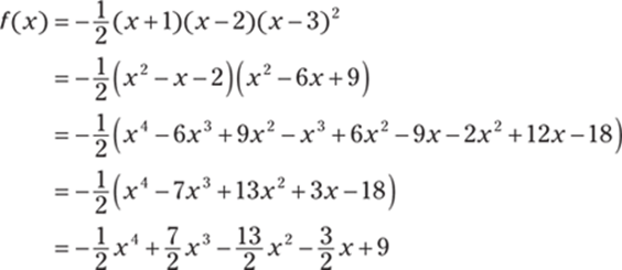
The polynomial is fourth-degree and has the x-intercepts at x = –1, 2, and 3, where 3 is a repeated root. Therefore, the polynomial has the factors (x + 1), (x – 2), and (x – 3)2, so you can write
![]()
Use the point (1, 4) to solve for a:
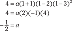
Now you can enter the value of a in the equation of the polynomial and simplify:
76. ![]()
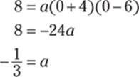
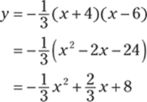
The parabola has x-intercepts at x = –4 and x = 6, so you know that (x + 4) and (x – 6) are factors of the parabola. Therefore, you can write
![]()
Use the point (0, 8) to solve for a:
Now you can enter the value of a in the equation of the parabola and simplify:
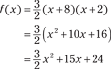
77. ![]()
The parabola has x-intercepts at x = –8 and x = –2, so you know that (x + 8) and (x + 2) are factors of the parabola. Therefore, you can write
![]()
Use the point (–4, –12) to solve for a:
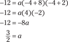
Now you can enter the value of a in the equation of the parabola and simplify:
78. domain: [–2, ∞); range: [1, ∞)
The function is continuous on its domain.
The lowest x coordinate occurs at the point (–2, 3), and then the graph extends indefinitely to the right; therefore, the domain is [–2, ∞). The lowest y coordinate occurs at the point (–1, 1), and then the graph extends indefinitely upward; therefore, the range is [1, ∞).
Note that the brackets in the interval notation indicate that the value –2 is included in the domain and that 1 is included in the range.
79. domain: [–5, 3]; range: [–2, 2]
Notice that the function is continuous on its domain.
The smallest x coordinate occurs at the point (–5, 0), and the largest x coordinate occurs at the point (3, 0); therefore, the domain is [–5, 3]. The smallest y coordinate occurs at the point (1, –2), and the largest y coordinate occurs at the point (–3, 2); therefore, the range is [–2, 2].
Note that the brackets in the interval notation indicate that the values –5 and 3 are included in the domain and that the values –2 and 2 are included in the range.
80. domain: ![]() ; range:
; range: ![]()
Notice that the function is continuous on its domain.
For the portion of the graph that's to the left of the y-axis, there's no largest x value due to the hole at (–1, –1); instead, the x values get arbitrarily close to –1. The graph then extends indefinitely to the left so that the domain for the left side of the graph is (–∞, –1). There's also no largest y value due to the hole at (–1, –1); the y values get arbitrarily close to –1. The graph then decreases as it approaches the horizontal asymptote at y = –3, so the range for this portion of the graph is (–3, –1).
For the portion of the graph that's to the right of the y-axis, the smallest x value is at the point (2, 2). The graph then extends indefinitely to the right, so the domain for the right side of the graph is [2, ∞). The smallest y value also occurs at the point (2, 2), and then the graph increases as it approaches the horizontal asymptote at y = 4; therefore, the range of this portion of the graph is [2, 4).
Putting the two parts together, the domain of the function is ![]() , and the range is
, and the range is ![]() .
.
81. ![]() ,
, ![]()
To determine the end behavior of a polynomial, you just have to determine the end behavior of the highest-powered term.
As x approaches –∞, you have

Note that even though the limit is approaching negative infinity, the limit is still positive due to the even exponent.
As x approaches ∞, you have

82. ![]() ,
, ![]()
To determine the end behavior of a polynomial, determine the end behavior of the highest-powered term.
As x approaches –∞, you have

Note that the limit is positive because a negative number raised to an odd power is negative, but after multiplying by –7, the answer becomes positive.
As x approaches ∞, you have

Likewise, the limit here is negative because a positive number raised to an odd power (or any power for that matter!) is positive, but after multiplying by –7, the answer becomes negative.
83. 3x + 12
Remove the parentheses and combine like terms:

84. 3x – 2
Remove the parentheses and combine like terms:

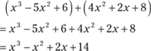
85. x3 – x2 + 2x + 14
Remove the parentheses and combine like terms:
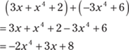
86. –2x4 + 3x + 8
Remove the parentheses and combine like terms:
87. x4 + 5x3 – 3x2
Remove the parentheses and combine like terms:

88. 3x – 7
Begin by removing the parentheses, being careful to distribute the –1 to the second term. Then collect like terms to simplify:

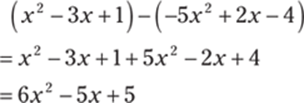
89. 6x2 – 5x + 5
Begin by removing the parentheses, being careful to distribute the –1 to the second term. Then collect like terms to simplify:
90. 4x3 + 5x2 – 8x + 14
Begin by removing the parentheses, being careful to distribute the –1 to the second term. Then collect like terms to simplify:

91. 2x2 + 3x + 1
Begin by removing the parentheses, being careful to distribute the –1 to the second and third terms. Then collect like terms to simplify:

92. 10x4 – 7x3 – 9x2 – 8x + 10
Begin by removing the parentheses, being careful to distribute the –1 to the second term. Then collect like terms to simplify:

93. 5x3 – 15x2
Distribute to get

94. 3x2 + 7x – 20
Distribute each term in the first factor to each term in the second factor. Then collect like terms:

95. x2y – xy2 + 6xy
Multiply each term in the first factor by xy:

96. 2x3 – 3x2 + 9x – 4
Distribute each term in the first factor to each term in the second factor and then collect like terms:
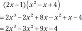
97. ![]()
Begin by distributing –x to each term in the second factor:

Next, multiply each term in the first factor by each term in the second factor:

98. ![]()
Using polynomial long division gives you
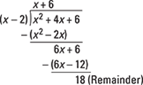
Remember to put the remainder over the divisor when writing the answer:
![]()
99. ![]()
Using polynomial long division gives you
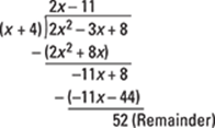
When writing the answer, put the remainder over the divisor:
![]()
100. ![]()
First add a placeholder for the missing x2 term in the numerator. Rewriting x3 – 2x + 6 as x3 + 0x2 – 2x + 6 will make all the like terms line up when you do the long division, making the subtraction a bit easier to follow.
Then use polynomial long division:
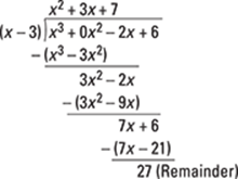
When you write the answer, put the remainder over the divisor:
![]()
101. ![]()
Begin by filling in all the missing terms so that everything will line up when you perform the long division. Here, add 0x3 and 0x as placeholders in the numerator and put 0x in the denominator:
![]()
Then use polynomial long division:
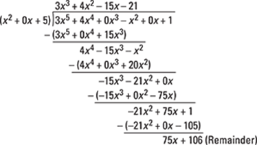
Put the remainder over the divisor when writing your answer:
![]()
102. ![]()
Begin by filling in all the missing terms so that everything will line up when you perform the long division:
![]()
Using polynomial long division gives you
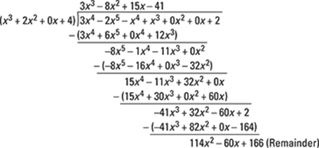
Then write your answer, putting the remainder over the divisor:
![]()
103. ![]() ;
; ![]() ;
; ![]()
When considering the sides of the right triangle, the values of the trigonometric functions are given by ![]() ,
,  , and
, and ![]() ; therefore,
; therefore,  ,
,  , and
, and ![]() .
.
104. ![]() ;
; ![]() ;
; ![]()
When considering the sides of the right triangle, the values of the trigonometric functions are given by ![]() ,
,  , and
, and ![]() ; therefore,
; therefore,  ,
,  , and
, and ![]() .
.
105. ![]()
You know the value of ![]() , so if you can find the value of
, so if you can find the value of ![]() , you can evaluate
, you can evaluate ![]() using
using ![]() . To find
. To find ![]() , use the identity
, use the identity ![]() :
:
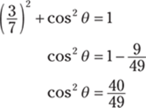
Next, take the square root of both sides, keeping the negative solution for cosine because ![]() :
:
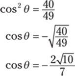
Therefore, using ![]() , you have
, you have

106. ![]()
To find the value of ![]() , you can find the value of
, you can find the value of ![]() and then use
and then use ![]() . Use the identity
. Use the identity ![]() to solve for
to solve for ![]() :
:
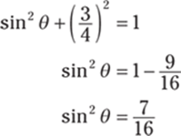
Next, take the square root of both sides, keeping the negative solution for sine because ![]() :
:

Therefore, using ![]() , you have
, you have

107. ![]()
To find the value of ![]() , you can use the identity
, you can use the identity ![]() . Notice that because
. Notice that because ![]() and
and ![]() , angle
, angle ![]() must be in the second quadrant. Using
must be in the second quadrant. Using ![]() , you can make a right triangle and find the missing side using the Pythagorean theorem. When making the triangle, you can neglect the negative sign:
, you can make a right triangle and find the missing side using the Pythagorean theorem. When making the triangle, you can neglect the negative sign:
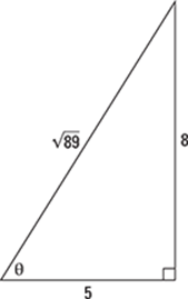
![]()
Because ![]() is in the second quadrant, you have
is in the second quadrant, you have ![]() and
and ![]() . Enter these values in the identity
. Enter these values in the identity ![]() and solve:
and solve:
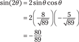
108. ![]()
To find the value of ![]() , you can use the identity
, you can use the identity ![]() . Using
. Using ![]() you can make a right triangle and find the missing side using the Pythagorean theorem. When making the triangle, you can neglect the negative sign:
you can make a right triangle and find the missing side using the Pythagorean theorem. When making the triangle, you can neglect the negative sign:

![]()
Now use the identity ![]() . The sine is negative, so you have
. The sine is negative, so you have ![]() :
:
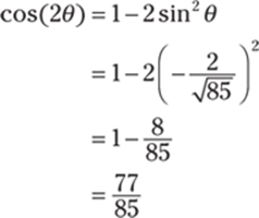
109. ![]() rad
rad
Because 180° = π rad, you have ![]() , so multiply the number of degrees by this value:
, so multiply the number of degrees by this value:
![]()
110. ![]() rad
rad
Because 180° = π rad, you have ![]() , so multiply the number of degrees by this value:
, so multiply the number of degrees by this value:
![]()
111. ![]() rad
rad
Because 180° = π rad, you have ![]() , so multiply the number of degrees by this value:
, so multiply the number of degrees by this value:
![]()
112. ![]() rad
rad
Because 180° = π rad, you have ![]() , so multiply the number of degrees by this value:
, so multiply the number of degrees by this value:
![]()
113. 210°
Because π rad = 180°, you have  , so multiply the number of radians by this value:
![]()
114. 165°
Because π rad = 180°, you have  , so multiply the number of radians by this value:
![]()
115. –108°
Because π rad = 180°, you have  , so multiply the number of radians by this value:
![]()
116. –630°
Because π rad = 180°, you have  , so multiply the number of radians by this value:
![]()
117. ![]()
Because ![]() is in Quadrant II and the angle is measured counterclockwise, you have
is in Quadrant II and the angle is measured counterclockwise, you have ![]() . Therefore,
. Therefore, ![]() is the most appropriate choice.
is the most appropriate choice.
118. ![]()
Because ![]() is in Quadrant III and the angle is measured clockwise, you have
is in Quadrant III and the angle is measured clockwise, you have ![]() . Therefore,
. Therefore, ![]() is the most appropriate choice.
is the most appropriate choice.
119. ![]()
Because ![]() is in Quadrant IV and the angle is measured counterclockwise, you have
is in Quadrant IV and the angle is measured counterclockwise, you have ![]() . Therefore,
. Therefore, ![]() is the most appropriate choice.
is the most appropriate choice.
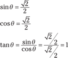
120. ![]() ;
; ![]() ;
; ![]()
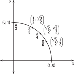
The given angle measure is ![]() . Using the first quadrant of the unit circle, you have the following:
. Using the first quadrant of the unit circle, you have the following:
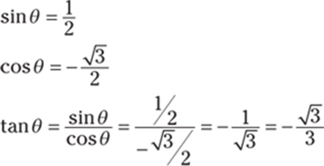
121. ![]() ;
; ![]() ;
; ![]()
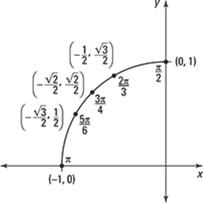
The given angle measure is ![]() . Using the second quadrant of the unit circle, you have the following:
. Using the second quadrant of the unit circle, you have the following:
122. ![]() ;
; ![]() ;
; ![]()
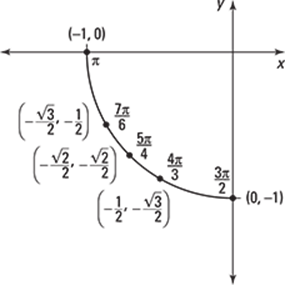
Use the third quadrant of the unit circle. Note that because the angle ![]() touches the unit circle in the same place as the angle
touches the unit circle in the same place as the angle ![]() , you have the following:
, you have the following:
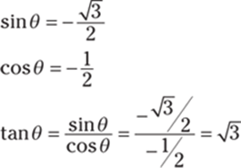
123. ![]() ;
; ![]() ;
; ![]()
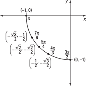
Use the third quadrant of the unit circle. The angle ![]() touches the unit circle in the same place as the angle
touches the unit circle in the same place as the angle ![]() , so you have the following:
, so you have the following:
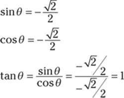
124. ![]() ;
; ![]() ;
; ![]()
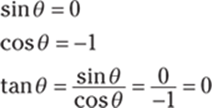
Because the angle ![]() intersects the unit circle at the point (–1, 0), you have the following:
intersects the unit circle at the point (–1, 0), you have the following:
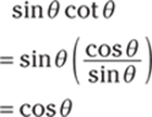
125. ![]()
Simply rewrite cotangent and simplify:
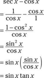
126. sin x tan x
Begin by writing sec x as ![]() . Then get common denominators and simplify:
. Then get common denominators and simplify:
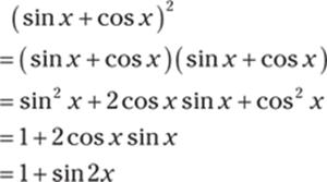
127. 1 + sin 2x
Expand the given expression and use the identity sin2 x + cos2 x = 1 along with 2 sin x cos x = sin(2x):
128. sin x
Use the identity sin(A – B) = sin A cos B – cos A sin B on the expression sin(π – x):
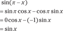
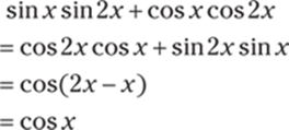
129. cos x
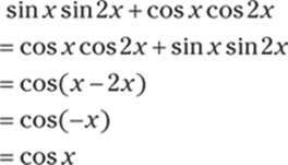
Use the identity cos A cos B + sin A sin B = cos(A – B) to get
Note that you can also use the following:
130. ![]()
First get common denominators:
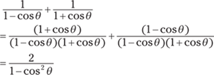
Then use the identity sin2 x = 1 – cos2 x in the denominator:
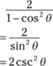
131. csc x + cot x
Begin by multiplying the numerator and denominator by the conjugate of the denominator, 1 + cos x. Then start to simplify:
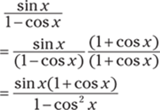
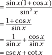
Continue, using the identity 1 – cos2 x = sin2 x to simplify the denominator:
132. ![]()
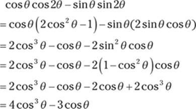
Use the identity cos(A + B) = cos A cos B – sin A sin B:

Then use the identities ![]() and
and ![]() and simplify:
and simplify:
133. ![]() ,
, ![]()
Solve for sin x:

The solutions are x = ![]() and
and ![]() in the interval [0, 2π].
in the interval [0, 2π].
134. 0, π, 2π
Make one side of the equation zero, use the identity ![]() , and then factor:
, and then factor:
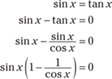
Setting the first factor equal to zero gives you sin x = 0, which has the solutions x = 0, π, and 2π. Setting the second factor equal to zero gives you ![]() so that cos x = 1, which has the solutions x = 0 and 2π.
so that cos x = 1, which has the solutions x = 0 and 2π.
135. ![]() , π,
, π, ![]()
Factor the equation:

Setting the first factor equal to zero gives you 2 cos x – 1 = 0 so that ![]() , which has the solutions
, which has the solutions ![]() and
and ![]() . Setting the second factor equal to zero gives you cos x + 1 = 0 so that cos x = –1, which has the solution x = π.
. Setting the second factor equal to zero gives you cos x + 1 = 0 so that cos x = –1, which has the solution x = π.
136. ![]() ,
, ![]() ,
, ![]() ,
, ![]()
To solve the equation ![]() , you must find the solutions to two equations: tan x = 1 and tan x = –1. For the equation tan x = 1, you have the solutions
, you must find the solutions to two equations: tan x = 1 and tan x = –1. For the equation tan x = 1, you have the solutions ![]() and
and ![]() . For the equation tan x = –1, you have the solutions
. For the equation tan x = –1, you have the solutions ![]() and
and ![]() .
.
137. ![]() ,
, ![]()
Factor the equation 2 sin2 x – 5 sin x – 3 = 0 to get
![]()
Setting the first factor equal to zero gives you 2 sin x + 1 = 0 so that ![]() , which has the solutions
, which has the solutions ![]() and
and ![]() . Setting the second factor equal to zero gives you sin x – 3 = 0 so that sin x = 3. Because 3 is outside the range of the sine function, this equation from the second factor has no solution.
. Setting the second factor equal to zero gives you sin x – 3 = 0 so that sin x = 3. Because 3 is outside the range of the sine function, this equation from the second factor has no solution.
138. ![]() ,
, ![]()
Begin by making one side of the equation equal to zero. Then use the identity ![]() and factor:
and factor:
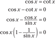
Setting the first factor equal to zero gives you cos x = 0, which has the solutions x = ![]() and
and ![]() . Setting the second factor equal to zero gives you
. Setting the second factor equal to zero gives you ![]() so that sin x = 1, which has the solution
so that sin x = 1, which has the solution ![]() .
.
139. ![]() ,
, ![]() ,
, ![]() ,
, ![]()
Begin by making the substitution 2x = y. Because 0 ≤ x ≤ 2π, it follows that 0 ≤ 2x ≤ 4π and that 0 ≤ y ≤ 4π.
Solving the equation ![]() gives you the solutions
gives you the solutions ![]() ,
, ![]() ,
, ![]() , and
, and ![]() in the interval [0, 4π].
in the interval [0, 4π].
Next, take each solution, set it equal to 2x, and solve for x: ![]() so that
so that ![]() ;
; ![]() so that
so that ![]() ;
; ![]() so that
so that ![]() ; and
; and ![]() so that
so that ![]() .
.
140. ![]() ,
, ![]() ,
, ![]() ,
, ![]()
Begin by making one side of the equation zero. Then use the identity sin 2x = 2 sin x cos x and factor:
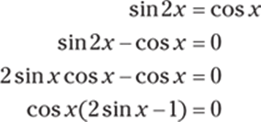
Setting the first factor equal to zero gives you cos x = 0, which has the solutions ![]() and
and ![]() . Setting the second factor equal to zero gives you 2 sin x – 1 = 0 so that
. Setting the second factor equal to zero gives you 2 sin x – 1 = 0 so that ![]() , which has the solutions
, which has the solutions ![]() and
and ![]() .
.
141. ![]() ,
, ![]()
Begin by using the identity ![]() and then factor:
and then factor:

Set each factor equal to zero and solve for x. The equation cos x = 0 has the solutions ![]() and
and ![]() , and the equation 1 + sin x = 0 gives you sin x = –1, which has the solution
, and the equation 1 + sin x = 0 gives you sin x = –1, which has the solution ![]() .
.
142. ![]() ,
, ![]() ,
, ![]()
Use the identity cos 2x = 2 cos2 x – 1, make one side of the equation zero, and factor:
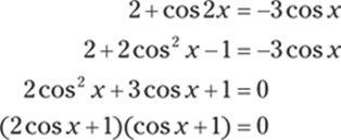
Set each factor equal to zero and solve for x. Setting the first factor equal to zerogives you 2 cos x + 1 = 0 so that ![]() , which has the solutions
, which has the solutions ![]() and
and ![]() . Setting the second factor equal to zero gives you cos x + 1 = 0 so that cos x = –1, which has the solution x = π.
. Setting the second factor equal to zero gives you cos x + 1 = 0 so that cos x = –1, which has the solution x = π.
143. ![]() ,
, ![]() ,
, ![]() ,
, ![]() ,
, ![]() ,
, ![]()
Begin by making the substitution y = 3x. Because 0 ≤ x ≤ 2π, you have 0 ≤ 3x ≤ 6π so that 0 ≤ y ≤ 6π. Finding all solutions of the equation tan y = –1 in the interval [0, 6π] gives you ![]() ,
, ![]() ,
, ![]() ,
, ![]() ,
, ![]() , and
, and ![]() .
.
Next, take each solution, set it equal to 3x, and solve for x: ![]() so that
so that ![]() ;
; ![]() so that
so that ![]() ;
; ![]() so that
so that ![]() ;
; ![]() so that
so that ![]() ;
; ![]() so that
so that ![]() ; and
; and ![]() so that
so that ![]() .
.
144. ![]() ,
, ![]() ,
, ![]() ,
, ![]()
Begin by making one side of the equation equal to zero and then factor:
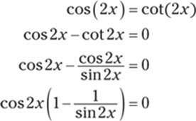
Next, make the substitution y = 2x:

Because 0 ≤ x ≤ 2π, it follows that 0 ≤ 2x ≤ 4π so that 0 ≤ y ≤ 4π.
Setting the first factor equal to zero gives you cos y = 0, which has the solutions ![]() ,
, ![]() ,
, ![]() , and
, and ![]() . Take each solution, set it equal to 2x, and solve for x:
. Take each solution, set it equal to 2x, and solve for x: ![]() so that
so that ![]() ;
; ![]() so that
so that ![]() ;
; ![]() so that
so that ![]() ; and
; and ![]() so that
so that ![]() .
.
Proceed in a similar manner for the second factor: ![]() so that sin y = 1, which has the solutions
so that sin y = 1, which has the solutions ![]() and
and ![]() . Now take each solution, set it equal to 2x, and solve for x:
. Now take each solution, set it equal to 2x, and solve for x: ![]() so that
so that ![]() , and
, and ![]() so that
so that ![]() .
.
145. amplitude: ![]() ; period: 2π; phase shift:
; period: 2π; phase shift: ![]() ; midline y = 0
; midline y = 0
For the function  , the amplitude is
 ![]() , the period is
, the period is ![]() , the phase shift is
, the phase shift is ![]() , and the midline is y = D. Writing
, and the midline is y = D. Writing  gives you the amplitude as
 ![]() , the period as
, the period as ![]() , the phase shift as
, the phase shift as ![]() , and the midline as y = 0.
, and the midline as y = 0.
146. amplitude: ![]() ; period: 2; phase shift:
; period: 2; phase shift: ![]() ; midline y = 0
; midline y = 0
For the function  , the amplitude is
 ![]() , the period is
, the period is ![]() , the phase shift is
, the phase shift is ![]() , and the midline is y = D. Writing
, and the midline is y = D. Writing  gives you the amplitude as
 ![]() , the period as
, the period as ![]() , the phase shift as
, the phase shift as ![]() , and the midline as y = 0.
, and the midline as y = 0.
147. amplitude: 3; period: 2; phase shift: ![]() ; midline y = 2
; midline y = 2
For the function  , the amplitude is
 ![]() , the period is
, the period is ![]() , the phase shift is
, the phase shift is ![]() , and the midline is y = D. Writing
, and the midline is y = D. Writing  gives you the amplitude as
 ![]() , the period as
, the period as ![]() , the phase shift as
, the phase shift as ![]() , and the midline as y = 2.
, and the midline as y = 2.
148. amplitude: 1; period: 4π; phase shift: –π; midline ![]()
For the function  , the amplitude is
 ![]() , the period is
, the period is ![]() , the phase shift is
, the phase shift is ![]() , and the midline is y = D. Writing
, and the midline is y = D. Writing ![]() gives you the amplitude as
gives you the amplitude as ![]() , the period as
, the period as  , the phase shift as –π, and the midline as
 ![]() .
.
149. f (x) = 2 sin(2x)
For the function  , the amplitude is
 ![]() , the period is
, the period is ![]() , the phase shift is
, the phase shift is ![]() , and the midline is y = D. The function has a period of π, so one possible value of B is B = 2. If you use a sine function to describe the graph, there's no phase shift, so you can use C = 0. The line y = 0 is the midline of the function so that D = 0. Last, the amplitude is 2, so you can use A = 2 because the function increases for values of x that are slightly larger than zero. Therefore, the function
, and the midline is y = D. The function has a period of π, so one possible value of B is B = 2. If you use a sine function to describe the graph, there's no phase shift, so you can use C = 0. The line y = 0 is the midline of the function so that D = 0. Last, the amplitude is 2, so you can use A = 2 because the function increases for values of x that are slightly larger than zero. Therefore, the function ![]() describes the given graph. Note that you can also use other functions to describe this graph.
describes the given graph. Note that you can also use other functions to describe this graph.
150. f (x) = 2 cos(2x)
For the function  , the amplitude is
 ![]() , the period is
, the period is ![]() , the phase shift is
, the phase shift is ![]() , and the midline is y = D. The function has a period of π, so one possible value of B is B = 2. If you use a cosine function to describe the graph, there's no phase shift; therefore, you can use C = 0. The line y = 0 is the midline of the function, so D = 0. Last, the amplitude is 2; you can use A = 2 because the function decreases for values of x that are slightly larger than zero. Therefore, the function f (x) = 2 cos(2x) describes the given graph. Note that you can also use other functions to describe this graph.
, and the midline is y = D. The function has a period of π, so one possible value of B is B = 2. If you use a cosine function to describe the graph, there's no phase shift; therefore, you can use C = 0. The line y = 0 is the midline of the function, so D = 0. Last, the amplitude is 2; you can use A = 2 because the function decreases for values of x that are slightly larger than zero. Therefore, the function f (x) = 2 cos(2x) describes the given graph. Note that you can also use other functions to describe this graph.
151. ![]()
For the function  , the amplitude is
 ![]() , the period is
, the period is ![]() , the phase shift is
, the phase shift is ![]() , and the midline is y = D. The function has a period of 4π, so one possible value of B is
, and the midline is y = D. The function has a period of 4π, so one possible value of B is ![]() . If you use a cosine function to describe the graph, there's no phase shift, so you can use C = 0. The line y = 0 is the midline of the function, so D = 0. Last, the amplitude is 2, so you can use A = –2 because the function increases for values of x that are slightly larger than zero. Therefore, the function
. If you use a cosine function to describe the graph, there's no phase shift, so you can use C = 0. The line y = 0 is the midline of the function, so D = 0. Last, the amplitude is 2, so you can use A = –2 because the function increases for values of x that are slightly larger than zero. Therefore, the function ![]() describes the given graph. Note that you can also use other functions to describe this graph.
describes the given graph. Note that you can also use other functions to describe this graph.
152. f (x) = 2 cos(2x) + 1
For the function  , the amplitude is
 ![]() , the period is
, the period is ![]() , the phase shift is
, the phase shift is ![]() , and the midline is y = D. The function has a period of π, so one possible value of B is B = 2. If you use a cosine function to describe the graph, there's no phase shift, so you can use C = 0. The line y = 1 is the midline of the function, so D = 1. Last, the amplitude is 2, so you can use A = 2 because the function decreases for values of x that are slightly larger than zero. Therefore, the function f (x) = 2 cos(2x) + 1 describes the given graph. Note that you can also use other functions to describe this graph.
, and the midline is y = D. The function has a period of π, so one possible value of B is B = 2. If you use a cosine function to describe the graph, there's no phase shift, so you can use C = 0. The line y = 1 is the midline of the function, so D = 1. Last, the amplitude is 2, so you can use A = 2 because the function decreases for values of x that are slightly larger than zero. Therefore, the function f (x) = 2 cos(2x) + 1 describes the given graph. Note that you can also use other functions to describe this graph.
153. ![]() For the function
For the function  , the amplitude is
 ![]() , the period is
, the period is ![]() , the phase shift is
, the phase shift is ![]() , and the midline is y = D. The function has a period of 4π, so one possible value of B is
, and the midline is y = D. The function has a period of 4π, so one possible value of B is ![]() . Think of the graph as a cosine graph that's flipped about the x-axis and shifted to the right; that means there's a phase shift of
. Think of the graph as a cosine graph that's flipped about the x-axis and shifted to the right; that means there's a phase shift of ![]() to the right, so
to the right, so ![]() . The line y = 0 is the midline of the function, so D = 0. Last, the amplitude is 2, so you can use A = –2 because the function increases for values of x that are slightly larger than
. The line y = 0 is the midline of the function, so D = 0. Last, the amplitude is 2, so you can use A = –2 because the function increases for values of x that are slightly larger than ![]() . Therefore, the following function describes the graph:
. Therefore, the following function describes the graph:
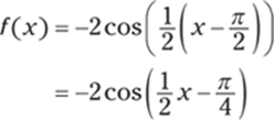
Note that you can also use other functions to describe this graph.
154. ![]()
For the function  , the amplitude is
 ![]() , the period is
, the period is ![]() , the phase shift is
, the phase shift is ![]() , and the midline is y = D. The function has a period of 4π, so one possible value of B is
, and the midline is y = D. The function has a period of 4π, so one possible value of B is ![]() . Think of the graph as a cosine graph that's flipped about the x-axis and shifted to the right and down; there's a phase shift of
. Think of the graph as a cosine graph that's flipped about the x-axis and shifted to the right and down; there's a phase shift of ![]() to the right so that
to the right so that ![]() . The line y = –1 is the midline of the function, so D = –1. Last, the amplitude is 2, so you can use A = –2 because the function increases for values of x that are slightly larger than
. The line y = –1 is the midline of the function, so D = –1. Last, the amplitude is 2, so you can use A = –2 because the function increases for values of x that are slightly larger than ![]() . Therefore, the following function describes the given graph.
. Therefore, the following function describes the given graph.
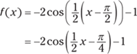
Note that you can also use other functions to describe this graph.
155. ![]()
To evaluate  , find the solution of
 ![]() , where
, where ![]() . Because
. Because ![]() , you have
, you have  .
.
156. ![]()
To evaluate arctan(–1) = x, find the solution of –1 = tan x, where ![]() . Because
. Because ![]() , you have
, you have ![]() .
.
157. ![]()
To evaluate  , first find the value of
 ![]() . To evaluate
. To evaluate ![]() , where
, where ![]() , find the solution of
, find the solution of ![]() . Because
. Because ![]() , you have
, you have ![]() . Therefore,
. Therefore,  .
.
158. ![]()
To evaluate  , first find the value of
  . To evaluate
  , where
 ![]() , find the solution of
, find the solution of ![]() . Because
. Because  , you have
  . Therefore,
  .
.
159. ![]()
The value of ![]() probably isn't something you've memorized, so to evaluate
probably isn't something you've memorized, so to evaluate ![]() , you can create a right triangle.
, you can create a right triangle.
Let ![]() so that
so that ![]() . Using
. Using ![]() , create the right triangle; then use the Pythagorean theorem to find the missing side:
, create the right triangle; then use the Pythagorean theorem to find the missing side:
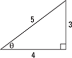
By the substitution, you have ![]() , and from the right triangle, you have
, and from the right triangle, you have ![]() .
.
160. ![]()
To evaluate ![]() , first create two right triangles using the substitutions tan−1(2) = α and tan−1(3) = β.
, first create two right triangles using the substitutions tan−1(2) = α and tan−1(3) = β.
To make the first right triangle, use tan−1(2) = α. You know that 2 = tan α, and you can find the missing side of the first right triangle using the Pythagorean theorem:

As for the second right triangle, because tan−1(3) = β, you know that 3 = tan β. Again, you can use the Pythagorean theorem to find the missing side of the right triangle:

The substitutions give you ![]() . Using a trigonometric identity, you know that sin(α + β) = sin α cos β + cos α sin β. From the right triangles, you can read off each of the values to get the following:
. Using a trigonometric identity, you know that sin(α + β) = sin α cos β + cos α sin β. From the right triangles, you can read off each of the values to get the following:
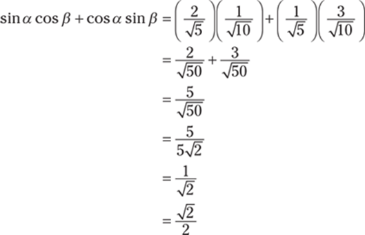
161. x = 0.412, π – 0.412
To solve sin x = 0.4 for x over the interval [0, 2π], begin by taking the inverse sine of both sides:

The other solution belongs to Quadrant II because the sine function also has positive values there:
![]()
162. x = 2.465, 2π – 2.456
To solve cos x = –0.78 for x over the interval [0, 2π], begin by taking the inverse cosine of both sides:

The other solution belongs to Quadrant III because the cosine function also has negative values there:
![]()
163. x = 0.322, ![]() , π + 0.322,
, π + 0.322, ![]()
To solve 5 sin(2x) + 1 = 4 for x over the interval [0, 2π], begin by isolating the term involving sine:
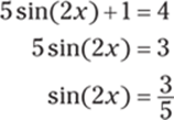
You can also use the substitution y = 2x to help simplify. Because 0 ≤ x ≤ 2π, it follows that 0 ≤ 2x ≤ 4π so that 0 ≤ y ≤ 4π. Use the substitution and take the inverse sine of both sides:
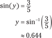
It follows that in the interval [0, 4π], 2π + 0.644 is also a solution because when you add 2π, the resulting angle lies at the same place on the unit circle.
Likewise, there's a solution to the equation ![]() in the second quadrant because the function also has positive values there, namely π – 0.644; adding 2π gives you the other solution, 3π – 0.644. Therefore, y = 0.644, π – 0.644, 2π + 0.644, and 3π – 0.644 are all solutions.
in the second quadrant because the function also has positive values there, namely π – 0.644; adding 2π gives you the other solution, 3π – 0.644. Therefore, y = 0.644, π – 0.644, 2π + 0.644, and 3π – 0.644 are all solutions.
Last, substitute 2x into the equations and divide to get the solutions for x:


The solutions are x = 0.322, ![]() , π + 0.322, and
, π + 0.322, and ![]() .
.
164. x = 0.321, ![]() ,
, ![]() ,
, ![]() ,
, ![]() , 2π – 0.321
, 2π – 0.321
To solve 7 cos(3x) – 1 = 3 for x over the interval [0, 2π], first isolate the term involving cosine:

You can also use the substitution y = 3x to simplify the equation. Because 0 ≤ x ≤ 2π, it follows that 0 ≤ 3x ≤ 6π so that 0 ≤ y ≤ 6π. Use the substitution and take the inverse cosine of both sides:
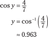
It follows that in the interval [0, 6π], y = 2π + 0.963 and y = 4π + 0.963 are also solutions because adding multiples of 2π makes the resulting angles fall at the same places on the unit circle.
Likewise, there's a solution to the equation ![]() in the fourth quadrant because cosine also has positive values there, namely y = 2π – 0.963. Because y = 2π – 0.963 is a solution, it follows that y = 4π – 0.963 and y = 6π – 0.963 are also solutions.
in the fourth quadrant because cosine also has positive values there, namely y = 2π – 0.963. Because y = 2π – 0.963 is a solution, it follows that y = 4π – 0.963 and y = 6π – 0.963 are also solutions.
Therefore, you have y = 0.963, 2π – 0.963, 2π + 0.963, 4π – 0.963, 4π + 0.963, and 6π – 0.963 as solutions to ![]() . Last, substitute 3x into the equations and divide to solve for x:
. Last, substitute 3x into the equations and divide to solve for x:


Therefore, the solutions are x = 0.321, ![]() ,
, ![]() ,
, ![]() ,
, ![]() , and 2π – 0.321.
, and 2π – 0.321.
165. x = π + 0.887, 2π – 0.887
To solve 2 sin2 x + 8 sin x + 5 = 0 for x over the interval [0, 2π], first use the quadratic formula:
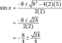
Simplifying gives you ![]() and
and ![]() .
.
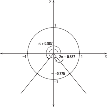
You now need to find solutions to sin x = –0.775 and sin x = –3.225. Notice that sin x = –3.225 has no solutions because –3.225 is outside the range of the sine function.
To solve sin x = –0.775, take the inverse sine of both sides:

Note that this solution isn't in the desired interval, [0, 2π]. The solutions in the given interval belong to Quadrants III and IV, respectively, because in those quadrants, the sine function has negative values; those solutions are x = π + 0.887 and x = 2π – 0.887.
166. x = π – 0.322, 2π – 0.322, ![]() ,
, ![]()
To solve 3 sec2 x + 4 tan x = 2 for x over the interval [0, 2π], begin by using the identity sec2 x = 1 + tan2 x and make one side of the equation equal to zero:
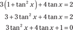
Next, use the quadratic formula to find tan x:
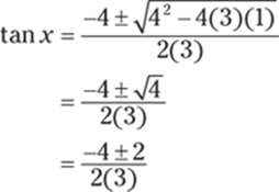
Therefore, tan x = –1 and ![]() .
.
The solutions to the equation tan x = –1 are ![]() and
and ![]() . To solve
. To solve ![]() , take the inverse tangent of both sides:
, take the inverse tangent of both sides:
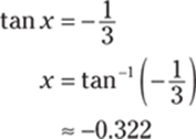
Note that this solution isn't in the given interval. The solutions that are in the given interval and belong to Quadrants II and IV (where the tangent function is negative) are x = π – 0.322 and x = 2π – 0.322.
167. 1
As x approaches 3 from the left, the y values approach 1 so that ![]() .
.
168. 3
As x approaches 3 from the right, the y values approach 3 so that ![]() .
.
169. 2
As x approaches –3 both from the left and from the right, the y values approach 2 so that ![]() .
.
Note that the actual value of f (–3) doesn't matter when you're finding the limit.
170. 3
As x approaches 1 from the left, the y values approach 3 so that ![]() .
.
171. 3
As x approaches 1 from the right, the y values approach 3 so that ![]() .
.
172. 5
As x approaches –2 both from the left and from the right, the y values approach 5 so that ![]() .
.
173. 4
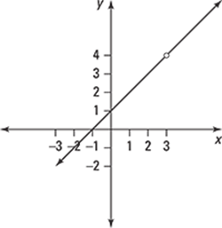
Note that substituting the limiting value, 3, into the function ![]() gives you the indeterminate form
gives you the indeterminate form ![]() .
.
To find the limit, first factor the numerator and simplify:
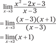
Then substitute 3 for x:
![]()
174. ![]()
Note that substituting the limiting value, 2, into the function ![]() gives you the indeterminate form
gives you the indeterminate form ![]() .
.
To find the limit, first factor the numerator and denominator and simplify:
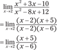
Then substitute 2 for x:

175. ![]()
Note that substituting the limiting value, –5, into the function ![]() gives you the indeterminate form
gives you the indeterminate form ![]() .
.
To find the limit, first factor the numerator and denominator and simplify:
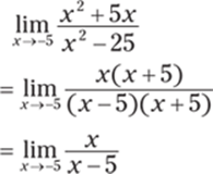
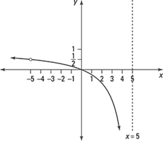
Then substitute –5 for x:
![]()
176. 4
Note that substituting the limiting value, 4, into the function ![]() gives you the indeterminate form
gives you the indeterminate form ![]() .
.
To find the limit, first factor the numerator and simplify:
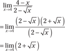
Then substitute 4 for x:
![]()
177. 1
Note that substituting in the limiting value, 0, gives you an indeterminate form. For example, as x approaches 0 from the right, you have the indeterminate form ∞ – ∞, and as x approaches 0 from the left, you have the indeterminate form –∞ + ∞.
To find the limit, first get common denominators and simplify:
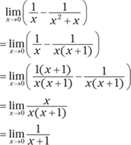
Then substitute 0 for x:
![]()
178. 0
The given function is continuous everywhere, so you can simply substitute in the limiting value:
![]()
179. 3
Note that substituting the limiting value, –1, into the function ![]() gives you the indeterminate form
gives you the indeterminate form ![]() .
.
To find the limit, first factor the numerator and simplify:
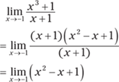
Then substitute –1 for x:
![]()
180. ![]()
Note that substituting the limiting value, 0, into the function ![]() gives you the indeterminate form
gives you the indeterminate form ![]() .
.
To find the limit, first multiply the numerator and denominator by the conjugate of the numerator and then simplify:
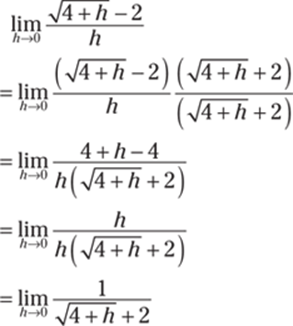
Then substitute 0 for h:
![]()
181. 108
Note that substituting the limiting value, 3, into the function ![]() gives you the indeterminate form
gives you the indeterminate form ![]() .
.
To find the limit, first factor the numerator and simplify:
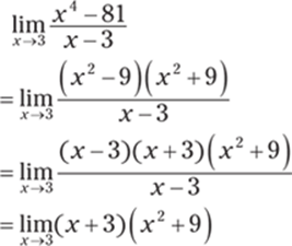
Then substitute 3 for x:
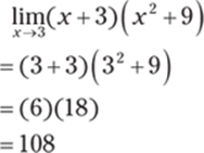
182. ∞
Note that substituting in the limiting value gives you an indeterminate form.
Because x is approaching 0 from the right, you have x > 0 so that ![]() . Therefore, the limit becomes
. Therefore, the limit becomes
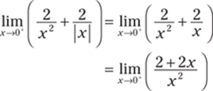
As x → 0+, you have (2 + 2x) → 2 and x2 → 0+ so that  . The limit is positive infinity because dividing 2 by a very small positive number close to zero gives you a very large positive number.
183. ∞
Note that substituting in the limiting value gives you the indeterminate form ∞ – ∞.
Because x is approaching 0 from the left, you have x < 0 so that ![]() . Therefore, the limit becomes
. Therefore, the limit becomes
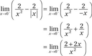
Now consider the numerator and denominator as x → 0–. As x → 0–, you have (2 + 2x) → 2 and x2 → 0+ so that  . The limit is positive infinity because dividing 2 by a very small positive number close to zero gives you a very large positive number.
184. limit does not exist
Note that substituting in the limiting value gives you the indeterminate form ![]() .
.
Examine both the left-hand limit and right-hand limit to determine whether the limits are equal. To find the left-hand limit, consider values that are slightly smaller than ![]() and substitute into the limit. Notice that to simplify the absolute value in the denominator of the fraction, you replace the absolute values bars with parentheses and add a negative sign, because substituting in a value less than
and substitute into the limit. Notice that to simplify the absolute value in the denominator of the fraction, you replace the absolute values bars with parentheses and add a negative sign, because substituting in a value less than ![]() will make the number in the parentheses negative; the extra negative sign will make the value positive again.
will make the number in the parentheses negative; the extra negative sign will make the value positive again.
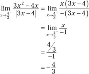
You deal with the right-hand limit similarly. Here, when removing the absolute value bars, you simply replace them with parentheses; you don't need the negative sign because the value in the parentheses is positive when you're substituting in a value larger than ![]() .
.
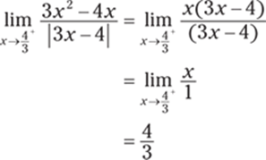
Because the right-hand limit doesn't equal the left-hand limit, the limit doesn't exist.
185. ![]()
Note that substituting the limiting value, 5, into the function ![]() gives you the indeterminate form
gives you the indeterminate form ![]() .
.
To find the limit, first factor the numerator and denominator and simplify:
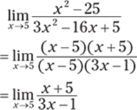
Then substitute 5 for x:
![]()
186. ![]()
Note that substituting in the limiting value gives you the indeterminate form ![]() .
.
Begin by multiplying the numerator and denominator of the fraction by the conjugate of the numerator:
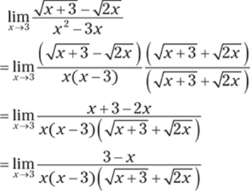
Next, factor –1 from the numerator and continue simplifying:
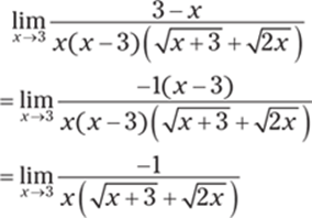
To find the limit, substitute 3 for x:
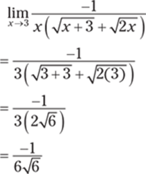
187. 12
Note that substituting the limiting value, 0, into the function  gives you the indeterminate form
 ![]() .
.
Expand the numerator and simplify:
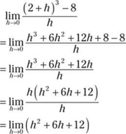
To find the limit, substitute 0 for h:
![]()
188. 1
Note that substituting in the limiting value, 4, gives you the indeterminate form ![]() .
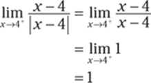
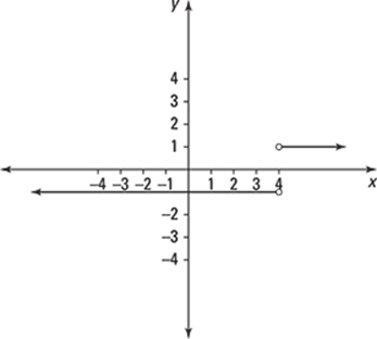
.
Because x is approaching 4 from the right, you have x > 4 so that ![]() . Therefore, the limit becomes
. Therefore, the limit becomes
189. –1
Note that substituting in the limiting value gives you the indeterminate form ![]() .
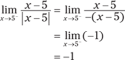
.
Because x is approaching 5 from the left, you have x < 5 so that ![]() . Therefore, the limit becomes
. Therefore, the limit becomes
190. ![]()
Note that substituting in the limiting value, –5, into the function  gives you the indeterminate form
 ![]() .
.
Begin by writing the two fractions in the numerator as a single fraction by getting common denominators. Then simplify:
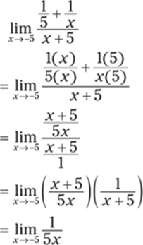
To find the limit, substitute –5 for x:
![]()
191. ![]()
Note that substituting in the limiting value gives you an indeterminate form. For example, as x approaches 0 from the right, you have the indeterminate form ∞ – ∞, and as x approaches 0 from the left, you have the indeterminate form –∞ + ∞.
Begin by getting common denominators:
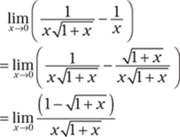
Next, multiply the numerator and denominator of the fraction by the conjugate of the numerator and simplify:
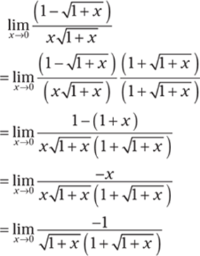
To find the limit, substitute 0 for x:
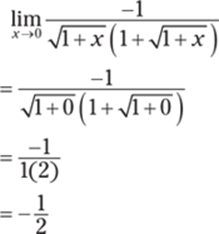
192. ![]()
Note that substituting in the limiting value, 0, gives you the indeterminate form ![]() .
.
Begin by rewriting the two terms in the numerator using positive exponents. After that, get common denominators in the numerator and simplify:
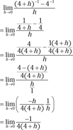
To find the limit, substitute 0 for h:
![]()
193. 5
The squeeze theorem states that if f (x) ≤ g(x) ≤ h(x) when x is near a (except possibly at a) and if ![]() , then
, then ![]() .
.
Note that ![]() and that
and that ![]() . Therefore, by the squeeze theorem,
. Therefore, by the squeeze theorem, ![]() .
.
194. 4
Note that ![]() and that
and that ![]() . Therefore, by the squeeze theorem,
. Therefore, by the squeeze theorem, ![]() .
.
195. 2
Note that ![]() and that
and that ![]() . Therefore, by the squeeze theorem,
. Therefore, by the squeeze theorem, ![]() .
.
196. 0
Notice that for all values of x except for x = 0, you have  due to the range of the cosine function. So for all values of x except for x = 0, you have

Because x is approaching 0 (but isn't equal to 0), you can apply the squeeze theorem:

Therefore, you can conclude that  .
.
197. 0
Notice that for all values of x > 0, you have  due to the range of the sine function. So for all values of x > 0, you have

Because x is approaching 0 (but isn't equal to 0), you can apply the squeeze theorem:

Therefore, you can conclude that  .
.
198. 0
Notice that for all values of x except for x = 0, you have ![]() due to the range of the sine function. So for all values of x except for x = 0, you have the following (after multiplying by –1):
due to the range of the sine function. So for all values of x except for x = 0, you have the following (after multiplying by –1):
![]()
You need to make the center expression match the given one,  , so do a little algebra. Adding 3 gives you
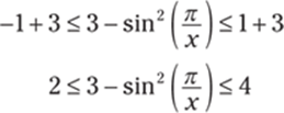
Now multiply by ![]() :
:

Note that ![]() for values of x greater than 0, so you don't have to flip the inequalities.
for values of x greater than 0, so you don't have to flip the inequalities.
Because the limit is approaching 0 from the right (but isn't equal to 0), you can apply the squeeze theorem to get

Therefore, you can conclude that  .
.
199. 5
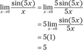
To use ![]() , you need the denominator of the function to match the argument of the sine. Begin by multiplying the numerator and denominator by 5. Then simplify:
, you need the denominator of the function to match the argument of the sine. Begin by multiplying the numerator and denominator by 5. Then simplify:
200. 0
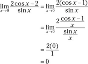
Factor the 2 from the numerator and then multiply the numerator and denominator by ![]() . Then simplify:
. Then simplify:
201. ![]()
Begin by using a trigonometric identity in the numerator and then factor:
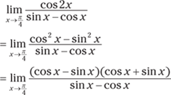
Next, factor out a –1 from the numerator and simplify:
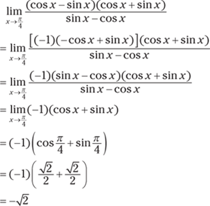
202. ![]()
You want to rewrite the expression so you can use ![]() . Begin by multiplying the numerator and denominator by
. Begin by multiplying the numerator and denominator by ![]() and rewrite the expression as the product of two fractions:
and rewrite the expression as the product of two fractions:
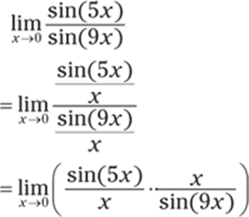
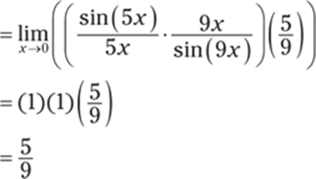
Now you want a 5 in the denominator of the first fraction and a 9 in the numerator of the second fraction. Multiplying by ![]() and also by
and also by ![]() gives you
gives you
203. ![]()
Begin by rewriting tan(7x) to get
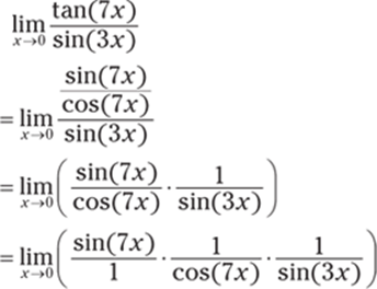
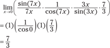
Now you want 7x in the denominator of the first fraction and 3x in the numerator of the third fraction. Therefore, multiply by ![]() ,
, ![]() , and
, and ![]() to get
to get
204. 8
Begin by breaking up the fraction as
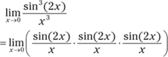
Next, you want each fraction to have a denominator of 2x, so multiply by ![]() ,
, ![]() , and
, and ![]() — or equivalently, by
— or equivalently, by ![]() — to get
— to get

205. ![]()
Begin by factoring the denominator and rewriting the limit:
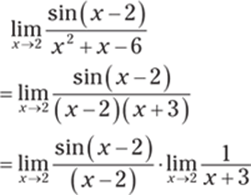
Notice that you can rewrite the first limit using the substitution ![]() so that as x → 2, you have
so that as x → 2, you have ![]() ; this step isn't necessary, but it clarifies how to use
; this step isn't necessary, but it clarifies how to use ![]() in this problem.
in this problem.
Replacing (x – 2) with ![]() and replacing x → 2 with
and replacing x → 2 with ![]() in the limit
in the limit ![]() gives you the following:
gives you the following:
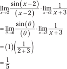
206. ![]()
Begin by rewriting tan x and then multiply the numerator and denominator by ![]() . Then simplify:
. Then simplify:
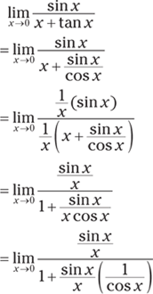
Then substitute 0 into the equation and solve:
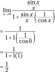
207. ∞
As x approaches 3 from the left, the y values approach ∞ so that ![]() .
.
208. –∞
As x approaches 3 from the right, the y values approach –∞ so that ![]() .
.
209. ∞
As x approaches 5 from the left, the y values approach ∞ so that ![]() .
.
210. –∞
As x approaches 5 from the right, the y values approach –∞ so that ![]() .
.
211. limit does not exist
As x approaches 5 from the left, the y values approach ∞. However, as x approaches 5 from the right, the y values approach –∞. Because the left-hand limit doesn't equal the right-hand limit, the limit doesn't exist.
212. ∞
As x approaches 1 from the right, you have (x – 1) → 0+ so that
![]()
Note that the limit is positive infinity because dividing 3 by a small positive number close to zero gives you a large positive number.
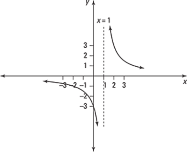
213. –∞
As x approaches 1 from the left, you have (x – 1) → 0– so that
![]()
Note that the limit is negative infinity because dividing 3 by a small negative number close to zero gives you a negative number whose absolute value is large.
214. –∞
Begin by writing the limit as  . Then consider what happens in the numerator and the denominator as x approaches
 ![]() from the right. As
from the right. As ![]() , you have sin x → 1 and cos x → 0–. Therefore, as
, you have sin x → 1 and cos x → 0–. Therefore, as ![]() , it follows that
, it follows that
![]()
215. ∞
Consider what happens in the numerator and denominator as x approaches π from the left. As x → π –, you have x2 → π2 and sin x → 0+. Therefore, as x → π –, it follows that
![]()
216. –∞
Consider what happens in the numerator and denominator as x approaches 5 from the left. As x → 5–, you have (x + 3) → 8 and (x – 5) → 0–. Therefore, as x → 5–, it follows that
![]()
217. –∞
Consider what happens in the numerator and denominator as x approaches 0 from the left. As x → 0–, you have (1 – x) → 1 and (ex – 1) → 0–. Therefore, as x → 0–, it follows that
![]()
218. –∞
Begin by writing ![]() . Then consider what happens in the numerator and denominator as x approaches 0 from the left. As x → 0–, you have cos x → 1 and sin x → 0–. Therefore, as x → 0–, it follows that
. Then consider what happens in the numerator and denominator as x approaches 0 from the left. As x → 0–, you have cos x → 1 and sin x → 0–. Therefore, as x → 0–, it follows that
![]()
219. ∞
Consider what happens in the numerator and denominator as x approaches 2. As x → 2, you have 4ex → 4e2 and ![]() . Therefore, as x → 2, it follows that
. Therefore, as x → 2, it follows that

220. –∞
Consider what happens to each factor in the numerator and denominator as x approaches ![]() from the right. As
from the right. As ![]() , you have
, you have ![]() and
and  . Therefore, as
 ![]() , it follows that
, it follows that

221. –∞
Consider what happens in the numerator and denominator as x approaches 5. As x → 5, you have sin x → sin 5, and because π < 5 < 2π, it follows that sin 5 < 0. And as x → 5, you also have (5 – x)4 → 0+. Therefore, as x → 5, it follows that

Note that the limit is negative infinity because sin(5) is negative, and dividing sin(5) by a small positive number close to zero gives you a negative number whose absolute value is large.
222. –∞
Consider what happens to each factor in the numerator and denominator as x approaches 0. You need to examine both the left-hand limit and the right-hand limit.
For the left-hand limit, as x → 0–, you have (x + 5) → 5, x4 → 0+, and (x – 6) → –6. Therefore, as x → 0–, it follows that

For the right-hand limit, you have (x + 5) → 5, x4 → 0+, and (x – 6) → –6. Therefore, as x → 0+, it follows that

Because the left-hand limit is equal to the right-hand limit,  .
.
223. limit does not exist
Begin by examining the left-hand limit and the right-hand limit to determine whether they're equal.
To find the limits, consider what happens in the numerator and denominator as x approaches 1. Using the left-hand limit, as x → 1–, you have (3x) → 3 and (ex – e) → 0–. Therefore, as x → 1–, it follows that
![]()
Using the right-hand limit, as x → 1+, you have (3x) → 3 and (ex – e) → 0+. So as x → 1+, it follows that
![]()
Because the left-hand limit doesn't equal the right-hand limit, the limit doesn't exist.
224. –∞
Consider what happens to each factor in the numerator and denominator as x approaches 0 from the right. You have (x – 1) → –1, x2 → 0+, and (x + 2) → 2. Therefore, as x → 0+, you get the following:

225. –∞
Consider what happens in the numerator and denominator as x approaches e from the left. As x → e–, you have x3 → e3 and (ln x – 1) → (ln e– – 1) → 0–. Therefore, as x → e–, it follows that
![]()
226. limit does not exist
Begin by examining both the left-hand limit and the right-hand limit to determine whether they're equal.
To find the limits, consider what happens in the numerator and denominator as x approaches e2. For the left-hand limit, as x → e2–, you have –x → –e2 and (ln x – 2) → 0–. Therefore, as x → e2–, it follows that
![]()
Note that the limit is positive infinity because dividing –e2 by a small negative number close to zero gives you a large positive number.
For the right-hand limit, as x → e2+, you have –x → –e2 and (ln x – 2) → 0+. Therefore, as x → e2+, it follows that
![]()
Because the left-hand limit doesn't equal the right-hand limit, the limit doesn't exist.
227. limit does not exist
Begin by examining the left-hand limit and the right-hand limit to determine whether they're equal.
To find the limits, consider what happens in the numerator and denominator as x approaches 2. For the left-hand limit, as x → 2–, you have (x + 2) → 4 and (x2 – 4) → 0–. Therefore, as x → 2–, it follows that
![]()
For the right-hand limit, as x → 2+, you have (x + 2) → 4 and (x2 – 4) → 0+. Therefore, as x → 2+, it follows that
![]()
Because the left-hand limit doesn't equal the right-hand limit, the limit doesn't exist.
228. limit does not exist
Begin by examining the left-hand limit and the right-hand limit to determine whether they're equal.
To find the limits, consider what happens in the numerator and denominator as x approaches 25. For the left-hand limit, as x → 25–, you have ![]() and (x – 25) → 0–. Therefore, as x → 25–, it follows that
and (x – 25) → 0–. Therefore, as x → 25–, it follows that

For the right-hand limit, as x → 25+, you have ![]() and (x – 25) → 0+. Therefore, as x → 25+, you have
and (x – 25) → 0+. Therefore, as x → 25+, you have

Because the left-hand limit doesn't equal the right-hand limit, the limit doesn't exist.
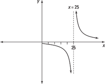
229. –∞
Consider what happens to each factor in the numerator and denominator as x approaches 0. As x → 0, you have (x2 + 4) → 4, x2 → 0+, and (x – 1) → –1. Therefore, as x → 0, it follows that

230. –∞
Consider what happens to each factor in the numerator and denominator as x approaches 0 from the left. You have (x – 1) → –1, x2 → 0+, and (x + 2) → 2. Therefore, as x → 0–, you get the following:

231. ∞
Consider what happens in the numerator and denominator as x approaches 3. As x → 3, you have (3 + x) → 6 and ![]() . Therefore, as x → 3, it follows that
. Therefore, as x → 3, it follows that

232. ![]()
As the x values approach –∞, the y values approach ![]() so that
so that ![]() .
.
233. ![]()
As the x values approach ∞, the y values approach ![]() so that
so that ![]() .
.
234. 2
As the x values approach –∞, the y values approach 2 so that ![]() .
.
235. 2
As the x values approach ∞, the y values approach 2 so that ![]() .
.
236. ![]()
Divide the numerator and denominator by the highest power of x that appears in the denominator, x1, and simplify:
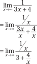
Then apply the limit:
![]()
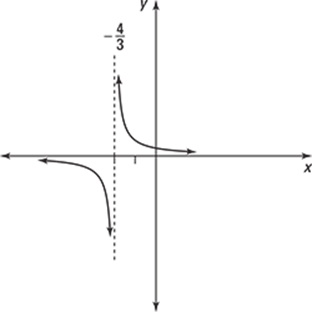
237. –∞
Begin by multiplying to get

For a polynomial function, the end behavior is determined by the term containing the largest power of x, so you have
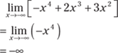
238. 3
Divide the numerator and denominator by the highest power of x that appears in the denominator, x1, and simplify:
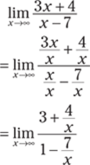
Then apply the limit:
![]()
239. limit does not exist
Because cos x doesn't approach a specific value as x approaches ∞, the limit doesn't exist.
240. 0
Begin by expanding the denominator:
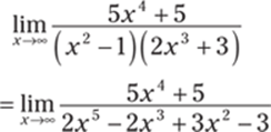
Next, divide the numerator and denominator by the highest power of x that appears in the denominator, x5, and simplify:
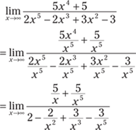
Then apply the limit:
![]()
241. ![]()
Begin by multiplying the numerator and denominator by ![]() so that you can simplify the expression underneath the square root:
so that you can simplify the expression underneath the square root:
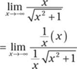
Because x is approaching –∞, you know that x < 0. So as you take the limit, you need to use the substitution  in the denominator. Therefore, you have
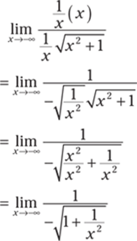
Now apply the limit:
![]()
242. ∞
Divide the numerator and denominator by the highest power of x that appears in the denominator, x2, and simplify:
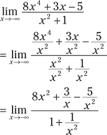
Then apply the limit. Consider what happens in the numerator and the denominator asx → –∞. In the numerator,  , and in the denominator,
  . Therefore, you have

243. ![]()
To simplify the expression underneath the radical, begin by multiplying the numerator and denominator by ![]() :
:
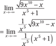
Because x is approaching –∞, you know that x < 0. So as you take the limit, you need to use the substitution  in the numerator:
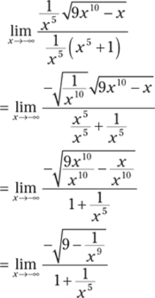
Now apply the limit:
![]()
244. ![]()
To simplify the expression underneath the radical, begin by multiplying the numerator and denominator by ![]() :
:
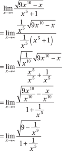
Now apply the limit:
![]()
245. –∞
Notice that if you consider the limit immediately, you have the indeterminate form ∞ – ∞.
Begin by factoring to get
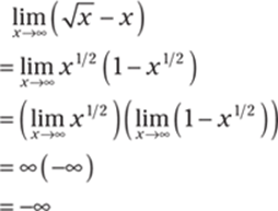
246. ![]()
Notice that if you consider the limit immediately, you have the indeterminate form ∞ – ∞.
Create a fraction and multiply the numerator and denominator by the conjugate of the expression ![]() . The conjugate is
. The conjugate is ![]() , so you have the following:
, so you have the following:
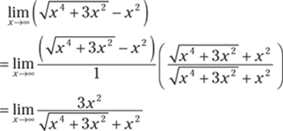
Next, multiply the numerator and denominator by ![]() so you can simplify the expression underneath the radical:
so you can simplify the expression underneath the radical:
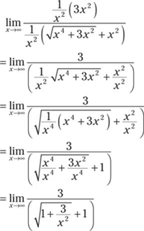
Now apply the limit:

247. ![]()
Notice that if you consider the limit immediately, you have the indeterminate form –∞ + ∞.
Create a fraction and multiply the numerator and denominator by the conjugate of the expression ![]() . The conjugate is
. The conjugate is ![]() , so you have
, so you have
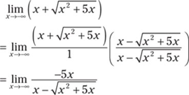
Next, multiply the numerator and denominator by ![]() so that you can simplify the expression underneath the square root:
so that you can simplify the expression underneath the square root:
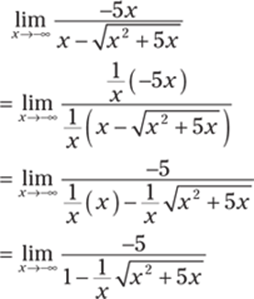
Because x is approaching –∞, you know that x < 0. So as you take the limit, you need to use the substitution  in the denominator. Therefore, you have
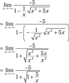
Now apply the limit:
![]()
248. ![]()
To find any horizontal asymptotes of the function ![]() , you need to consider the limit of the function as x → ∞ and as x → –∞. For the limit as x → ∞, begin by multiplying the numerator and denominator by
, you need to consider the limit of the function as x → ∞ and as x → –∞. For the limit as x → ∞, begin by multiplying the numerator and denominator by ![]() :
:
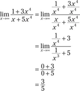
To find the limit as x → –∞, you can proceed in the same way in order to simplify:
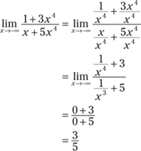
Therefore, the only horizontal asymptote is ![]() .
.
249. y = –1
To find any horizontal asymptotes of the function ![]() , you need to consider the limit of the function as x → ∞ and as x → –∞. For the limit as x → ∞, begin by multiplying the numerator and denominator by
, you need to consider the limit of the function as x → ∞ and as x → –∞. For the limit as x → ∞, begin by multiplying the numerator and denominator by ![]() :
:
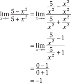
To find the limit as x → –∞, proceed in the same way:
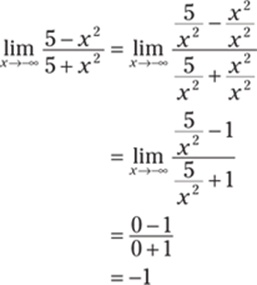
Therefore, the only horizontal asymptote is y = –1.
250. ![]()
In order to find any horizontal asymptotes of the function  , you need to consider the limit of the function as x → ∞ and as x → –∞. For the limit as x → ∞, begin by multiplying the numerator and denominator by
 ![]() :
:
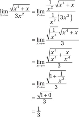
In order to find the limit as x → –∞, proceed in the same way, noting that as x → –∞, you still use  :
:
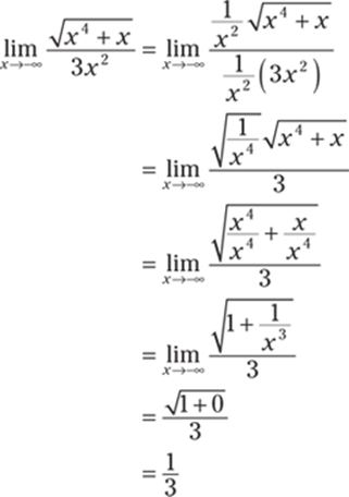
Therefore, the only horizontal asymptote is ![]() .
.
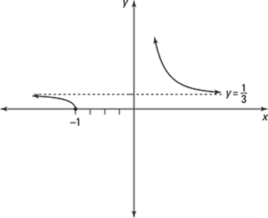
251. y = 1 and y = –1
To find any horizontal asymptotes of the function ![]() , you need to consider the limit of the function as x → ∞ and as x → –∞. For the limit as x → ∞, begin by multiplying the numerator and denominator by
, you need to consider the limit of the function as x → ∞ and as x → –∞. For the limit as x → ∞, begin by multiplying the numerator and denominator by ![]() :
:
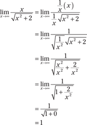
To find the limit as x → –∞, proceed in the same way, noting that as ![]() , you need to use the substitution
, you need to use the substitution  :
:
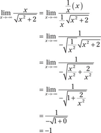
Therefore, the function has the horizontal asymptotes y = 1 and y = –1.
252. removable discontinuity at x = –3, jump discontinuity at x = 3
The limit exists at x = –3 but isn't equal to f (–3), which corresponds to a removable discontinuity.
At x = 3, the left-hand limit doesn't equal the right-hand limit (both limits exist as finite values); this corresponds to a jump discontinuity.
253. removable discontinuity at x = 1, infinite discontinuity at x = 5
The limit exists at x = 1, but f (1) is undefined, which corresponds to a removable discontinuity.
At x = 5, the left-hand limit is ∞ and the right-hand limit is –∞, so an infinite discontinuity exists at x = 5.
254. jump discontinuity at x = –2, jump discontinuity at x = 3
At x = –2, the left-hand limit doesn't equal the right-hand limit (both limits exist as finite values), which corresponds to a jump discontinuity.
At x = 3, the left-hand limit again doesn't equal the right-hand limit (both limits exist as finite values), so this also corresponds to a jump discontinuity.
255. removable discontinuity at x = –1, jump discontinuity at x = 4, infinite discontinuity at x = 6
At x = –1, the left-hand limit equals the right-hand limit, but the limit doesn't equal f (–1), which is undefined. Therefore, a removable discontinuity is at x = –1.
At x = 4, the left-hand limit doesn't equal the right-hand limit (both limits exist as finite values), so a jump discontinuity is at x = 4.
At x = 6, both the left and right-hand limits equal ∞, so an infinite discontinuity is at x = 6.
256. not continuous, infinite discontinuity
A function f (x) is continuous at x = a if it satisfies the equation ![]() . The left-hand limit at a is given by
. The left-hand limit at a is given by ![]() . As x → 2–, you have (x – 2) → 0– so that
. As x → 2–, you have (x – 2) → 0– so that ![]() . Because the discontinuity is infinite, you don't need to examine the right-hand limit; you can conclude that the function is not continuous.
. Because the discontinuity is infinite, you don't need to examine the right-hand limit; you can conclude that the function is not continuous.
257. continuous, f (a) = 2
A function f (x) is continuous at x = a if it satisfies the equation ![]() . The left-hand limit at a is
. The left-hand limit at a is ![]() , and the right-hand limit at a is
, and the right-hand limit at a is ![]() . The left-hand and right-hand limits match, so the limit at a exists and is equal to 2.
. The left-hand and right-hand limits match, so the limit at a exists and is equal to 2.
The value at a is ![]() . Because the function satisfies the definition of continuity, you can conclude that that function is continuous at a = 1.
. Because the function satisfies the definition of continuity, you can conclude that that function is continuous at a = 1.
258. continuous, f (a) = 5
A function f (x) is continuous at x = a if it satisfies the equation ![]() . The left-hand limit at a is
. The left-hand limit at a is
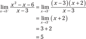
And the right-hand limit at a is
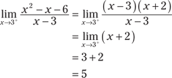
Note that in this case, you could have simply evaluated the limit as x approaches 3 instead of examining the left-hand limit and right-hand limit separately.
The left-hand and right-hand limits match, so the limit exists and is equal to 5. Because f (a) = f (3) = 5, the definition of continuity is satisfied and the function is continuous.
259. continuous, ![]()
A function f (x) is continuous at x = a if it satisfies the equation ![]() . The left-hand limit at a is
. The left-hand limit at a is
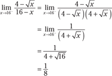
The right-hand limit at a is
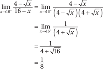
The left-hand and right-hand limits match, so the limit exists.
Note that in this case, you could have simply evaluated the limit as x approaches 16 instead of examining the left-hand limit and right-hand limit separately.
The value at a is given by ![]() , which matches the limit. Because the definition of continuity is satisfied, you can conclude that that function is continuous at a = 16.
, which matches the limit. Because the definition of continuity is satisfied, you can conclude that that function is continuous at a = 16.
260. not continuous, jump discontinuity
A function f (x) is continuous at x = a if it satisfies the equation ![]() . The left-hand limit at a is
. The left-hand limit at a is
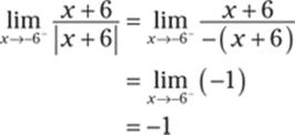
The right-hand limit at a is
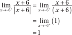
Because the left- and right-hand limits exist but aren't equal to each other, there's a jump discontinuity at a = –6.
261. not continuous, removable discontinuity
A function f (x) is continuous at x = a if it satisfies the equation ![]() . The left-hand limit at a is
. The left-hand limit at a is
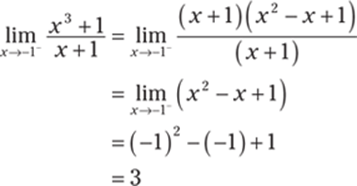
The right-hand limit at a is
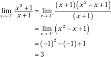
The left-hand and right-hand limits match, so the limit exists and is equal to 3.
Note that in this case, you could have simply evaluated the limit as x approaches –1 instead of examining the left-hand limit and right-hand limit separately.
However, because f (a) = f (–1) = 2, the function is not continuous; it has a removable discontinuity.
262. continuous at a = 0 and at a = π
A function f (x) is continuous at x = a if it satisfies the equation ![]() . To determine whether the function is continuous at a = 0, see whether it satisfies the equation
. To determine whether the function is continuous at a = 0, see whether it satisfies the equation ![]() . The left-hand limit at a = 0 is
. The left-hand limit at a = 0 is ![]() , and the right-hand limit at a = 0 is
, and the right-hand limit at a = 0 is ![]() . Because f (0) = 2 cos(0) = 2, the function is continuous at a = 0.
. Because f (0) = 2 cos(0) = 2, the function is continuous at a = 0.
Likewise, decide whether the function satisfies the equation ![]() . The left-hand limit at a = π is
. The left-hand limit at a = π is ![]() , and the right-hand limit at a = π is
, and the right-hand limit at a = π is ![]() . Because
. Because ![]() , the function is also continuous at a = π.
, the function is also continuous at a = π.
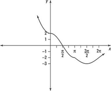
263. jump discontinuity at a = 1 and at a = 3
A function f (x) is continuous at x = a if it satisfies the equation ![]() . To determine whether the function is continuous at a = 1, see whether it satisfies the equation
. To determine whether the function is continuous at a = 1, see whether it satisfies the equation ![]() . The left-hand limit at a = 1 is
. The left-hand limit at a = 1 is ![]() , and the right-hand limit at a= 1 is
, and the right-hand limit at a= 1 is ![]() . The limits differ, so there's a jump discontinuity.
. The limits differ, so there's a jump discontinuity.
Likewise, decide whether the function satisfies the equation ![]() . The left-hand limit at a = 3 is
. The left-hand limit at a = 3 is ![]() , and the right-hand limit at a = 3 is
, and the right-hand limit at a = 3 is ![]() , so there's another jump discontinuity.
, so there's another jump discontinuity.
264. continuous at a = 2, jump discontinuity at a = 3
A function f (x) is continuous at x = a if it satisfies the equation ![]() . To determine whether the function is continuous at a = 2, see whether it satisfies the equation
. To determine whether the function is continuous at a = 2, see whether it satisfies the equation ![]() . The left-hand limit at a = 2 is
. The left-hand limit at a = 2 is ![]() , and the right-hand limit ata = 2 is
, and the right-hand limit ata = 2 is ![]() . Because
. Because ![]() , the func-tion is continuous at
, the func-tion is continuous at ![]() .
.
Likewise, decide whether the function satisfies the equation ![]() . The left-hand limit at a = 3 is
. The left-hand limit at a = 3 is ![]() , and the right-hand limit at a = 3 is
, and the right-hand limit at a = 3 is ![]() . The limits don't match, so there's a jump discontinuity at a = 3.
. The limits don't match, so there's a jump discontinuity at a = 3.
265. infinite discontinuity at a = 0, continuous at a = 4
A function f (x) is continuous at x = a if it satisfies the equation ![]() . To determine whether the function is continuous at a = 0, see whether it satisfies the equation
. To determine whether the function is continuous at a = 0, see whether it satisfies the equation ![]() . The left-hand limit at a = 0 is
. The left-hand limit at a = 0 is ![]() , and the right-hand limit at a= 0 is
, and the right-hand limit at a= 0 is ![]() , so there's an infinite discontinuity at a = 0.
, so there's an infinite discontinuity at a = 0.
Likewise, decide whether the function satisfies the equation ![]() . The left-hand limit at a = 4 is
. The left-hand limit at a = 4 is ![]() , and the right-hand limit at a = 4 is
, and the right-hand limit at a = 4 is ![]() . Because
. Because ![]() , the function is continuous at a = 4.
, the function is continuous at a = 4.
266. ![]()
To determine the value of c, you must satisfy the definition of a continuous function: ![]() .
.
The left-hand limit at x = 2 is given by ![]() , and the right-hand limit is given by
, and the right-hand limit is given by ![]() . Also note that f (2) = 2c – 2.
. Also note that f (2) = 2c – 2.
The left-hand limit must equal the right-hand limit, so set them equal to each other and solve for c:
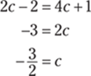
Therefore, ![]() is the solution.
is the solution.
267. c = 2
To determine the value of c, you must satisfy the definition of a continuous function: ![]() .
.
The left-hand limit at x = 4 is given by ![]() , and the right-hand limit is given by
, and the right-hand limit is given by ![]() . Also note that
. Also note that ![]() .
.
The left-hand limit must equal the right-hand limit, so set them equal to each other:
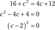
Therefore, c – 2 = 0, which gives you the solution c = 2.
268. [1, 2]
Recall the intermediate value theorem: Suppose that f is continuous on the closed interval [a, b], and let N be any number between f (a) and f (b), where f (a) ≠ f (b). Then a number c exists in (a, b) such that f (c) = N.
Notice that ![]() is a polynomial that's continuous everywhere, so the interme-diate value theorem applies. Checking the endpoints of the interval [1, 2] gives you
is a polynomial that's continuous everywhere, so the interme-diate value theorem applies. Checking the endpoints of the interval [1, 2] gives you

Because the function changes signs on this interval, there's at least one root in the interval by the intermediate value theorem.
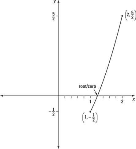
269. [16, 25]
Notice that ![]() is a continuous function for x ≥ 0, so the intermediate value theorem applies. Checking the endpoints of the interval [16, 25] gives you
is a continuous function for x ≥ 0, so the intermediate value theorem applies. Checking the endpoints of the interval [16, 25] gives you

Because the function changes signs on this interval, there's at least one root in the interval by the intermediate value theorem.
270. [2, 3]
The function f (x) = 2(3x) + x2 – 4 is continuous everywhere, so the intermediate value theorem applies. Checking the endpoints of the interval [2, 3] gives you

The number 32 is between 18 and 59, so by the intermediate value theorem, there exists at least one point c in the interval [2, 3] such that f (c) = 32.
271. [3, 4]
The function ![]() is continuous everywhere, so the intermediate value theorem applies. Checking the endpoints of the interval [3, 4] gives you
is continuous everywhere, so the intermediate value theorem applies. Checking the endpoints of the interval [3, 4] gives you

The number 22 is between 17 and 25, so by the intermediate value theorem, there exists at least one point c in the interval [3, 4] such that f (c) = 22.
272. x = 1
The graph has a point of discontinuity at x = 1, so the graph isn't differentiable there. However, the rest of the graph is smooth and continuous, so the derivative exists for all other points.
273. differentiable everywhere
Because the graph is continuous and smooth everywhere, the function is differentiable everywhere.
274. x = –2, x = 0, x = 2
The graph of the function has sharp corners at x = –2, x = 0, and x = 2, so the function isn't differentiable there.
You can also note that for each of the points x = –2, x = 0, and x = 2, the slopes of the tangent lines jump from 1 to –1 or from –1 to 1. This jump in slopes is another way to recognize values of x where the function is not differentiable.
275. ![]() , where n is an integer
, where n is an integer
Because y = tan x has points of discontinuity at ![]() , where n is an integer, the function isn't differentiable at those points.
, where n is an integer, the function isn't differentiable at those points.
276. x = 0
The tangent line would be vertical at x = 0, so the function isn't differentiable there.
277. 2
Use the derivative definition with f (x) = 2x – 1 and f (x + h) = 2(x + h) – 1 = 2x + 2h – 1: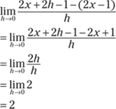
278. 2 x
Use the derivative definition with f (x) = x2 and f (x + h) = (x + h)2 = (x + h)(x + h) = x2 + 2xh + h2: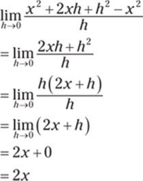
279. 1
Use the derivative definition with f (x) = 2 + x and f (x + h) = 2 + (x + h):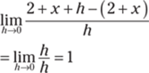
280. ![]()
Use the derivative definition with![]() and with
and with![]() to get the following:
to get the following: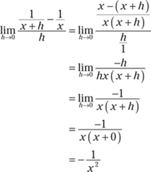
281. 3 x2 – 2x
Using the derivative definition with f (x) = x3 – x2 and with
gives you the following: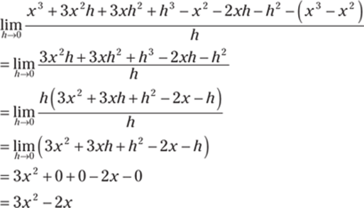
282. 6 x + 4
Using the derivative definition with f (x) = 3x2 + 4x and with
gives you the following: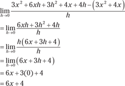
283. ![]()
Using the derivative definition with ![]() and with
and with ![]() gives you the following:
gives you the following: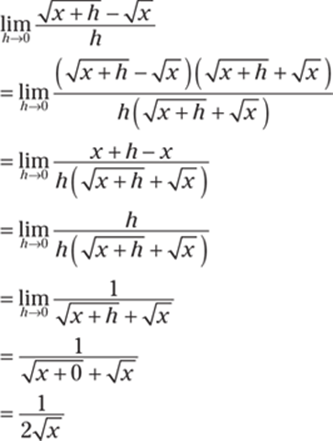
284. ![]()
Using the derivative definition with ![]() and with
and with ![]() gives you the following:
gives you the following: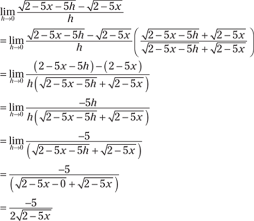
285. 
Use the derivative definition with ![]() and with
and with ![]() :
: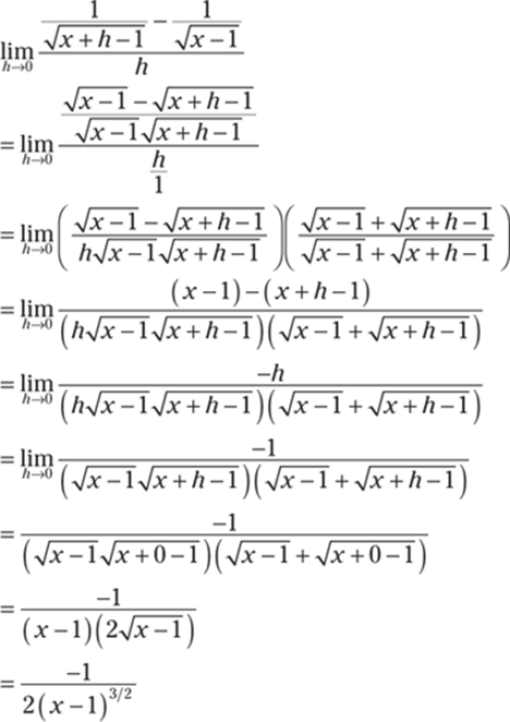
286. 3 x2 + 3
Use the derivative definition with f (x) = x3 + 3x and with f (x + h) = (x + h)3 + 3(x + h) = x3 + 3x2h + 3xh2 + h3 + 3x + 3h:
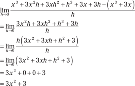
287. 
Using the derivative definition with ![]() and with
and with  gives you the following:
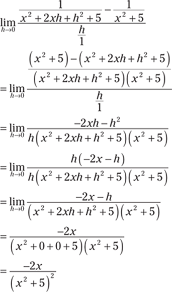
288. 
Using the derivative definition with ![]() and with
and with ![]() gives you the following:
gives you the following: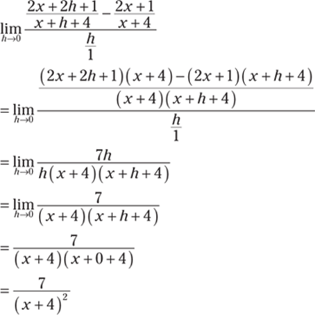
289. 
Using the derivative definition with ![]() and with
and with  gives you the following:
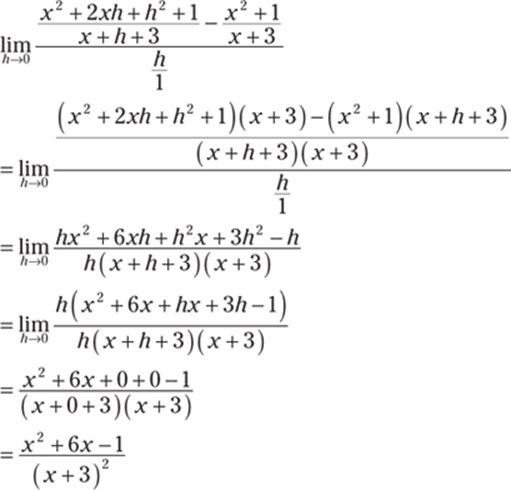
290. 
Using the derivative definition with ![]() and with
and with ![]() gives you
gives you 
To rationalize the numerator, consider the formula a3 – b3 = (a – b)(a2 + ab + b2). If you let a = (2x + 2h + 1)1/3 and b = (2x + 1)1/3, you have (a – b) in the numerator; that means you can rationalize the numerator by multiplying by (a2 + ab + b2):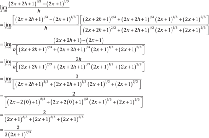
291. 0
The tangent line at x = 3 is horizontal, so the slope is zero. Therefore, f'(3) = 0.
292. –1
The slope of the tangent line at x = –1 is equal to –1, so f'(–1) = –1.
293. 1
The slope of the tangent line at x = –3 is equal to 1, so f'(–3) =1.
294. 3
The slope of the tangent line at any point on the graph of y = 3x + 4 is equal to 3, so f'(–22π3) = 3.
295. f'(1) < f'(–2) < f'(–3)
The tangent line at x = –3 has a positive slope, the slope of the tangent line at x = –2 is equal to zero, and the slope of the tangent line at x = 1 is negative. Therefore, f'(1) < f'(–2) < f'(–3).
296. f'(1) < f'(2) < 0.1 < f'(5)
The slope of the tangent line at x = 1 is negative, the slope of the tangent line at x = 2 is equal to zero, and the slope of the tangent line at x = 5 is clearly larger than 0.1. Therefore, f'(1) < f'(2) < 0.1 < f'(5).
297. 5
Use basic derivative rules to get f'(x) = 5.
298. 2 x + 3
Apply the power rule to each term, recalling that the derivative of a constant is zero: f'(x) = 2x + 3.
299. 4 x + 7
Begin by multiplying the two factors together:
Then apply the power rule to get the derivative:
300. 0
Because π3 is constant, f'(x) = 0.
301. ![]()
Split up the radical and rewrite the power on the variable using exponential notation:![]()
Then apply the power rule to find the derivative:
302. ![]()
Begin by breaking up the fraction: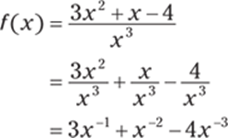
Then apply the power rule to find the derivative:
303. ![]()
Begin by multiplying the factors together: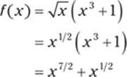
Then apply the power rule to find the derivative:
304. 
Begin by rewriting the function using a negative exponent:
Then apply the power rule to each term to get the derivative:
305. ![]()
Apply the power rule to the first two terms of ![]() , recalling that the derivative of a constant is zero:
, recalling that the derivative of a constant is zero: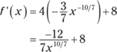
306. ![]()
Multiply the factors and rewrite the function using exponential notation: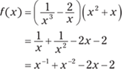
Next, apply the power rule to find the derivative:
307. ![]()
Begin by multiplying the factors together: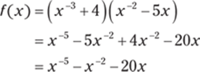
Then find the derivative using the power rule:
308. 16 x3 – 2x + 8
Apply the power rule to each term, recalling that the derivative of a constant is zero: f'(x) = 16x3 – 2x + 8.
309. 
Rewrite the function using exponential notation: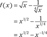
Then apply the power rule to each term to find the derivative: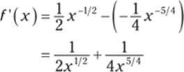
310. ![]() , 1
, 1
Begin by finding the derivative of the function f (x) = x3 – x2 – x + 1:![]()
A horizontal tangent line has a slope of zero, so set the derivative equal to zero, factor, and solve for x:
Setting each factor equal to zero gives you 3x + 1 = 0, which has the solution ![]() , and gives you x – 1 = 0, which has the solution x = 1.
, and gives you x – 1 = 0, which has the solution x = 1.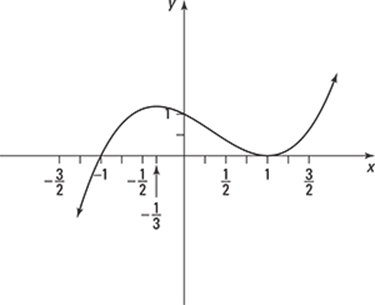
311. ![]()
Begin by finding the derivative of the function:![]()
Next, set the derivative equal to 6 and solve for x: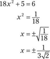
312. 16 x7 + 5x4 – 8x3 – 1
Recall that the product rule states ![]()
You can multiply out the expression f (x) = (2x3 + 1)(x5 – 1) first and then avoid using the product rule, but here's how to find the derivative using the product rule:
313. x(2 sin x + x cos x)
Applying the product rule to f (x) = x2 sin x gives you
314. ![]()
Apply the product rule to f (x) = sec x tan x:
315. (sec x)(1 + x tan x)
Begin by rewriting the original expression as ![]() and then apply the product rule:
and then apply the product rule:
316. 4 (csc x)(1 – x cot x)
Apply the product rule to f (x) = 4x csc x to get
317. 12
According to the product rule, ![]()
To find (fg)'(4), enter the numbers and solve:
318. 
Recall that the product rule states ![]()
You can apply the quotient rule directly, or you can rewrite the original function as ![]() and then apply the product rule to get the following:
and then apply the product rule to get the following:
319. x sec x tan x + 2 sec3 x
Apply the product rule to f (x) = sec x(x + tan x) as follows: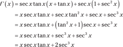
320. ![]()
Apply the product rule to f (x) = (x2 + x)csc x to get

321. 4 x2 (sec x)(3 + x tan x)
Applying the product rule to f (x) = 4x3 sec x gives you

322. ![]()
You can apply the quotient rule directly, or you can rewrite the original function as ![]() and then apply the product rule as follows:
and then apply the product rule as follows:
323. ![]()
Using the product rule on f (x) = x2g (x) and then factoring gives you the derivative as follows:
324. ![]()
Begin by breaking up the fraction and simplifying: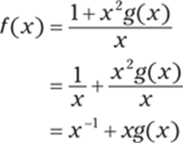
Next, apply the power rule to the first term and the product rule to the second term:
325. –46
The product rule tells you that ![]()
To find (fg)'(3), enter the numbers and solve:
326. 2 x cos x sin x – x2 sin2 x + x2 cos2 x
Recall that the product rule states ![]()
You can group the factors however you want and then apply the product rule within the product rule. If you group together the trigonometric functions and apply the product rule, you have f (x) = x2(cos x sin x) so that 
327. 
Begin by simplifying the given expression:
Then apply the product rule to the second term and the power rule to the first term:
328. 
Rewrite the original expression:
Then apply the product rule to get the derivative:
329. ![]()
First simplify the given function: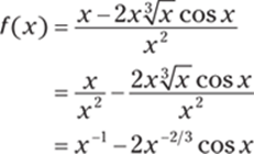
Then apply the product rule to find the derivative:
330. ![]()
You can use the quotient rule directly, or you can rewrite the original expression as ![]() and then apply the product rule as follows:
and then apply the product rule as follows:
331. ![]()
To find the derivative of ![]() , use the product rule within the product rule:
, use the product rule within the product rule:
332. 
Recall that the quotient rule states 
Apply the quotient rule to ![]() :
: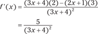
333. 
Apply the quotient rule to ![]() to get the derivative:
to get the derivative: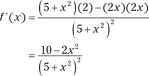
334. 
Apply the quotient rule to ![]() :
:
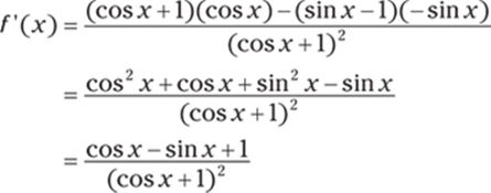
335. 
Apply the quotient rule to ![]() to get the following:
to get the following: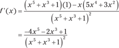
336. ![]()
The quotient rule gives you 
To find  , enter the numbers and solve:
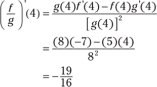
337. 
Recall that the quotient rule states 
Apply the quotient rule to ![]() :
: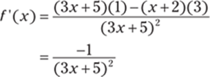
338. 
Apply the quotient rule to ![]() to find the derivative:
to find the derivative: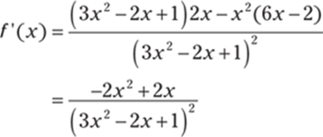
339. ![]()
Apply the quotient rule to ![]() to get the derivative:
to get the derivative: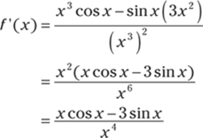
340. 
First, simplify the numerator and denominator:![]()
Then apply the quotient rule to get 
341. 
Apply the quotient rule to ![]() to get the following:
to get the following:
342. 
Apply the quotient rule to ![]() :
:
343. ![]()
The quotient rule says that 
To find  , enter the numbers and solve:
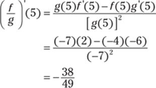
344. 
Recall that the quotient rule states 
Apply the quotient rule to  to get
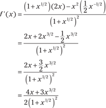
345. 
Apply the quotient rule to ![]() to get the following:
to get the following: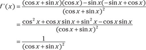
346. 
Apply the quotient rule to  :
: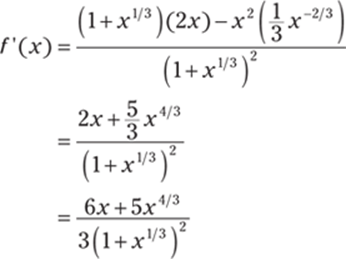
347. 
Apply the quotient rule to  to get
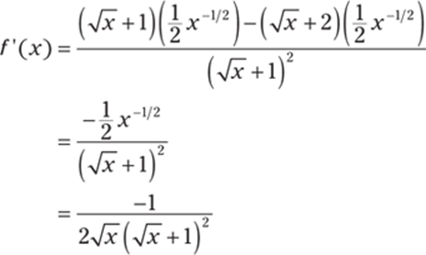
348. 
Apply the quotient rule to ![]() as follows:
as follows: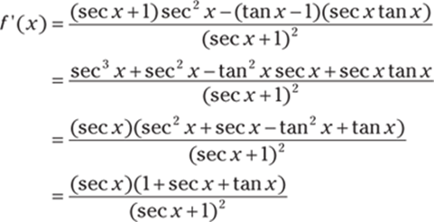
Note that the identity sec2 x – tan2 x = 1 was used to simplify the final expression.
349. 
First multiply the numerator and denominator by x: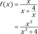
Then use the quotient rule to find the derivative: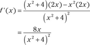
350. 
Applying the quotient rule to ![]() , followed by factoring and simplifying, gives you the following:
, followed by factoring and simplifying, gives you the following: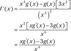
351. 
Applying the quotient rule to ![]() gives you
gives you 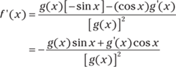
352. ![]()
Recall that the chain rule states ![]()
Applying the chain rule to ![]() gives you
gives you 
353. 4 cos(4x)
Apply the chain rule to f (x) = sin(4x):
354. 
Rewrite the function using exponential notation:![]()
Then apply the chain rule:
355. 
Rewrite the function as 
Then apply the chain rule to get the derivative: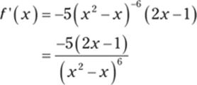
356. 
First rewrite the function:
Then apply the chain rule: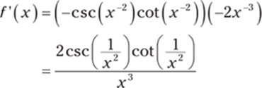
357. ![]()
Apply the chain rule to ![]() to get
to get 
358. 
Recall that the chain rule states ![]()
and that the quotient rule states 
To find the derivative of  , apply the quotient rule along with the chain rule:
359. ![]()
Recall that the chain rule states ![]()
and that the product rule states ![]()
To find the derivative of f (x) = cos(x sin x), apply the chain rule and the product rule:
360. ![]()
Rewrite the function using exponential notation:
Now apply the product rule, being careful to use the chain rule when taking the derivative of the second factor: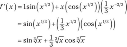
361. 
Recall that the chain rule states ![]()
and that the quotient rule states 
Rewrite the function using exponential notation: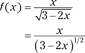
Next, apply the quotient rule, making sure to use the chain rule when taking the derivative of the denominator: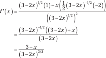
362. 4 sec2 x tan x
First rewrite the function:![]()
Applying the chain rule gives you the derivative:
363. 
Recall that the chain rule states ![]()
and that the quotient rule states 
Rewrite the function using exponential notation: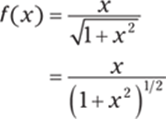
Apply the quotient rule and the chain rule to get the derivative: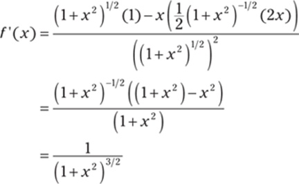
364. 
Recall that the chain rule states ![]()
and that the product rule states ![]()
Rewrite the function using exponential notation:
Then apply the product rule and also use the chain rule on the second factor to get the derivative: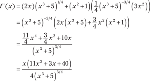
365. ![]()
To find the derivative of ![]() , use the product rule along with the chain rule and then factor:
, use the product rule along with the chain rule and then factor:
366. 
Recall that the chain rule states ![]()
and that the quotient rule states 
Applying the quotient rule and the chain rule to  gives you the following derivative:
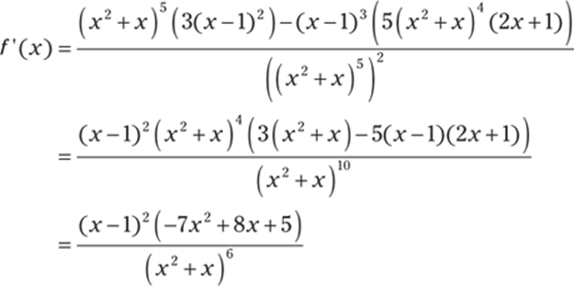
367. 
First rewrite the function using exponential notation:
Then apply both the chain rule and the quotient rule: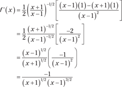
368. ![]()
To find the derivative of ![]() , apply the chain rule repeatedly:
, apply the chain rule repeatedly:
369. 
Rewrite the function using exponential notation:
Then apply the chain rule repeatedly to get the derivative: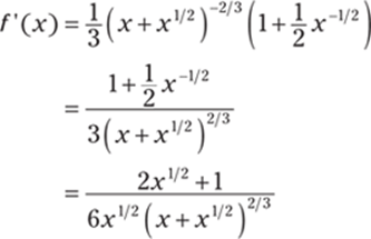
370. ![]()
Recall that the chain rule states ![]()
and that the product rule states ![]()
Applying the product rule and chain rule to f (x) = (1 + 5x)4(2 + x – x2)7 and then factoring (factoring can be the tricky part!) gives you the following:
371. x = 0, π, 2π
Recall that the chain rule states ![]()
Begin by finding the derivative of the function f (x) = 2 cos x + sin2 x:
Then set the derivative equal to zero to find the x values where the function has a horizontal tangent line:![]()
Next, set each factor equal to zero and solve for x: sin x = 0 has the solutions x = 0, π, 2π, and cos x – 1 = 0, or cos x = 1, has the solutions x = 0, 2π. The slope of the tangent line is zero at each of these x values, so the solutions are x = 0, π, 2π.
372. 
To find the derivative of ![]() , use the chain rule:
, use the chain rule: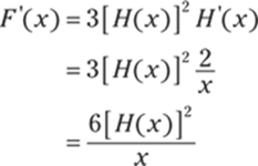
373. 28
Because the chain rule gives you ![]() , it follows that
, it follows that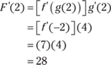
374. –40
Because the chain rule gives you ![]() , it follows that
, it follows that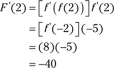
375. ![]()
Recall that the chain rule states ![]()
Using the chain rule on f (x) = H(x3) gives you the following:![]()
Because ![]() , you know that that
, you know that that ![]() , so the derivative becomes
, so the derivative becomes 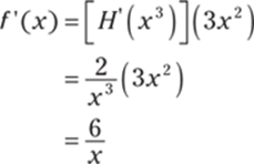
376. 80
Because the chain rule gives you ![]() , it follows that
, it follows that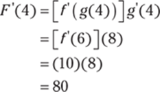
377. ![]()
Use properties of logarithms to rewrite the function:![]()
Then take the derivative:![]()
378. 
To find the derivative of f (x) = (ln x)4, apply the chain rule: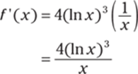
379. ![]()
Begin by using properties of logarithms to rewrite the function: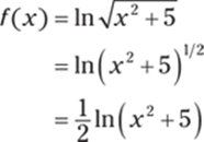
Then apply the chain rule to find the derivative: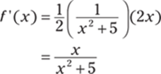
380. 
Begin by writing the function using exponential notation:
Then use the chain rule to find the derivative: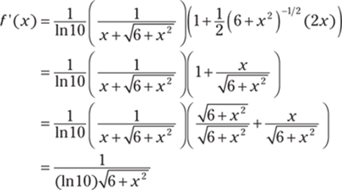
381. ![]()
To make the derivative easier to find, use properties of logarithms to break up the function:
Now apply the chain rule to each term to get the derivative:
382. ![]()
Begin by rewriting the function using properties of logarithms: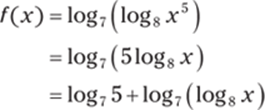
The derivative becomes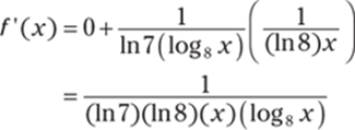
Note that log75 is a constant, so its derivative is equal to zero.
You can further simplify by using the change of base formula to write ![]() :
: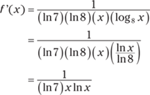
383. sec x
Applying the chain rule to ![]() gives you
gives you
384. 
To find the derivative of  , apply the quotient rule and chain rule to the first term and apply the chain rule to the second term:
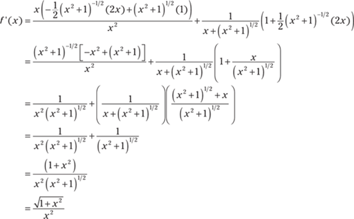
385. 
Begin by using properties of logarithms to rewrite the function: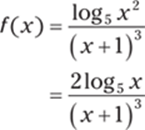
Then apply the quotient rule and the chain rule: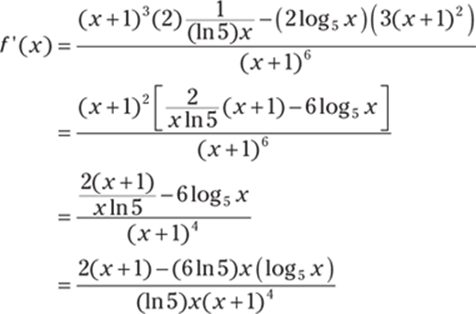
You can now further simplify by using the change of base formula to write ![]() so that you have
so that you have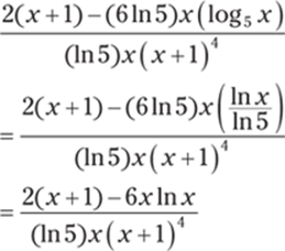
386. 
Begin by rewriting the function and taking the natural logarithm of each side: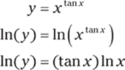
Take the derivative of each side with respect to x:![]()
Then multiply both sides by y:
Finally, replacing y with xtan x gives you the answer:
387. ![]()
Begin by rewriting the function and taking the natural logarithm of each side: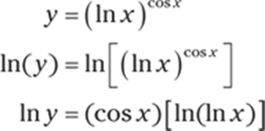
Then take the derivative of each side with respect to x:
Multiplying both sides by y produces
And replacing y with ![]() gives you the answer:
gives you the answer:![]()
388. 
Begin by rewriting the function and taking the natural logarithm of each side: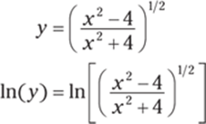
Using properties of logarithms to expand gives you
Next, take the derivative of each side with respect to x:
Multiplying both sides by y produces the following:
Replacing y with  and simplifying gives you the solution:
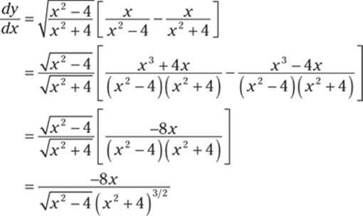
Note that you can find the derivative without logarithmic differentiation, but using it makes the math easier.
389. 
Begin by rewriting the function and taking the natural logarithm of each side: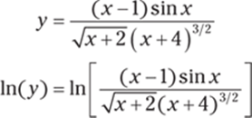
Use properties of logarithms to expand:![]()
Then take the derivative of each side with respect to x:
Multiplying both sides by y produces
Replacing with y with  gives you the answer:
Note that you can find the derivative without logarithmic differentiation, but using this technique makes the calculations easier.
390. 5 e5x
Apply the chain rule to find the derivative of f (x) = e5x:
391. ![]()
Applying the chain rule to ![]() gives you
gives you![]()
392. ![]()
Applying the product rule to ![]() gives you the derivative as follows:
gives you the derivative as follows:
393. 2 x
Use properties of logarithms to simplify the function:![]()
The derivative is simply equal to ![]()
394. ![]()
To find the derivative of ![]() , apply the product rule while also applying the chain rule to the first factor:
, apply the product rule while also applying the chain rule to the first factor:
395. 
Put the radical in exponential form:
Then apply the product rule as well as the chain rule to the first factor to get the derivative:
396. ![]()
Applying the chain rule to ![]() gives you the derivative as follows:
gives you the derivative as follows:
397. ![]()
Use properties of logarithms to break up the function:
Then apply the chain rule to each term to get the derivative:
398. 
Apply the quotient rule to find the derivative of ![]() :
: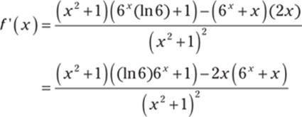
399. 
First rewrite the function:![]()
Applying the chain rule gives you the derivative as follows: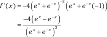
400. 
To find the derivative of ![]() , apply the quotient rule while applying the chain rule to the numerator:
, apply the quotient rule while applying the chain rule to the numerator: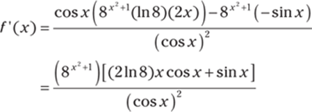
401. ![]()
To find the derivative of ![]() , apply the product rule while applying the chain rule to the second factor:
, apply the product rule while applying the chain rule to the second factor:
402. y = πx + 3
You can begin by finding the y value, because it isn't given:![]()
Next, find the derivative of the function:![]()
Substitute in the given x value to find the slope of the tangent line:![]()
Now use the point-slope formula for a line to get the tangent line at x = 0:
403. y = x + 1
Begin by finding the derivative of the function f (x) = x2 – x + 2:![]()
Substitute in the given x value to find the slope of the tangent line:![]()
Now use the point-slope formula for a line to get the tangent line at (1, 2):
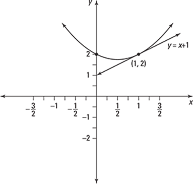
404. ![]()
You can begin by finding the y value, because it isn't given:![]()
Next, find the derivative of the function:
Substitute in the given x value to find the slope of the tangent line:
Now use the point-slope formula for a line to get the tangent line at x = 2:
405. ![]()
The normal line is perpendicular to the tangent line. Begin by finding the derivative of the function f (x) = 3x2 + x – 2:![]()
Then substitute in the given x value to find the slope of the tangent line:![]()
To find the slope of the normal line, take the opposite reciprocal of the slope of the tangent line to get ![]() .
.
Now use the point-slope formula for a line to get the normal line at (3, 28):
406. ![]()
The normal line is perpendicular to the tangent line. You can begin by finding the y value at ![]() , because it isn't given:
, because it isn't given:
Next, find the derivative of the function:![]()
Then substitute in the given x value to find the slope of the tangent line:
To find the slope of the normal line, take the opposite reciprocal of the slope of the tangent line to get –1.
Now use the point-slope formula for a line to get the normal line at ![]() :
:
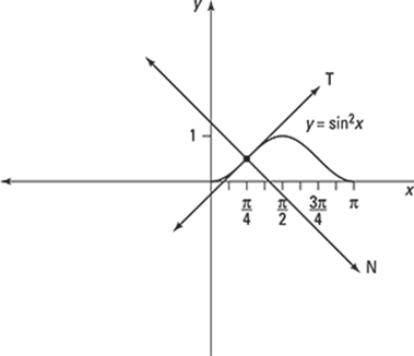
407. ![]()
The normal line is perpendicular to the tangent line. You can begin by finding the y value at x = e2, because it isn't given:![]()
Next, find the derivative of the function:![]()
Then substitute in the given x value to find the slope of the tangent line:![]()
To find the slope of the normal line, take the opposite reciprocal of the slope of the tangent line to get ![]() .
.
Now use the point-slope formula for a line to get the normal line at x = e2:
408. ![]()
Taking the derivative of both sides of x2 + y2 = 9 and solving for ![]() gives you the following:
gives you the following: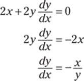
409. 
Take the derivative of both sides of y5 + x2y3 = 2 + x2y and solve for ![]() :
: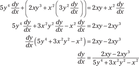
410. 
Take the derivative of both sides of x3y3 + x cos(y) = 7 and solve for ![]() :
: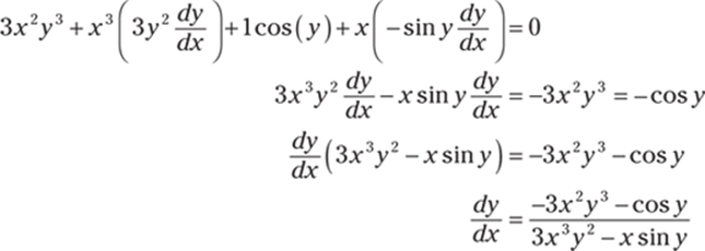
411. 
Take the derivative of both sides of ![]() and solve for
and solve for ![]() :
: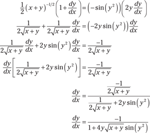
412. 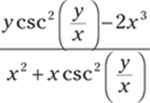
Take the derivative of both sides of  and solve for
 ![]() :
:
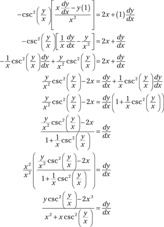
413. 
Take the derivative of both sides of ![]() and solve for
and solve for ![]() :
: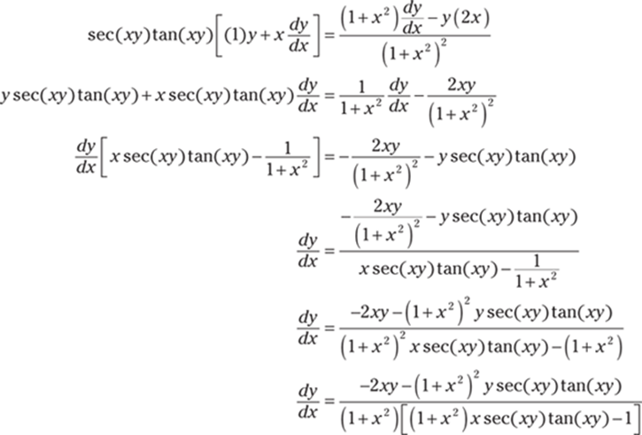
414. ![]()
Begin by finding the first derivative of 8x2 + y2 = 8: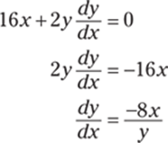
Next, find the second derivative:
Substituting in the value of ![]() gives you
gives you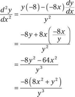
And now using 8x2 + y2 = 8 gives you the answer:
415. 
Begin by finding the first derivative of x5 + y5 = 1: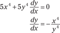
Next, find the second derivative:
Substituting in the value of  gives you
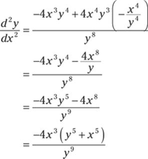
And now using x5 + y5 = 1 gives you the answer:
416. ![]()
Begin by finding the first derivative of x3 + y3 = 5: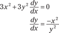
Next, find the second derivative:
Substituting in the value of  gives you
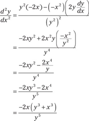
And now using x3 + y3 = 5 gives you the answer:
417. ![]()
Begin by finding the first derivative of ![]() :
: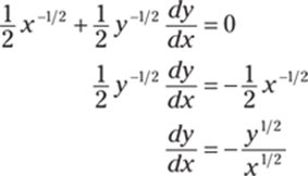
Next, find the second derivative:
Substituting in the value of  gives you
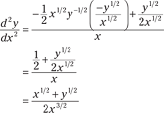
And now using ![]() gives you the answer:
gives you the answer:
418. y = –x + 2
You know a point on the tangent line, so you just need to find the slope. Begin by finding the derivative of x2 + xy + y2 = 3: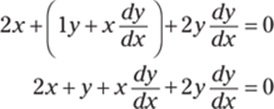
Next, enter the values x = 1 and y = 1 and solve for the slope ![]() :
: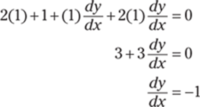
The tangent line has a slope of –1 and passes through (1, 1), so its equation is
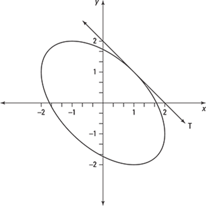
419. ![]()
You know a point on the tangent line, so you just need to find the slope. Begin by finding the derivative of 3(x2 + y2)2 = 25(x2 – y2):
Then enter the values x = 2 and y = 1 and solve for the slope ![]() :
: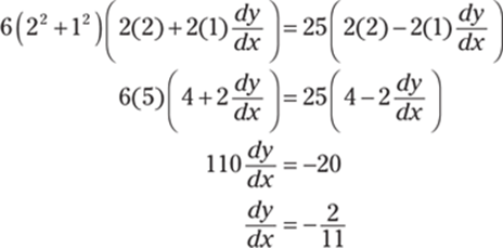
The tangent line has a slope of ![]() and passes through (2, 1), so its equation is
and passes through (2, 1), so its equation is
420. y = –x + 1
You know a point on the tangent line, so you just need to find the slope. Begin by taking the derivative of x2 + 2xy + y2:
Then use the values x = 0 and y = 1 and solve for the slope ![]() :
: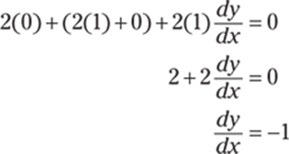
The tangent line has a slope of –1 and passes through (0, 1), so its equation is
421. ![]()
You know a point on the tangent line, so you just need to find the slope. Begin by taking the derivative of cos(xy) + x2 = sin y: 
Then use the values x = 1 and ![]() and solve for the slope
and solve for the slope ![]() :
: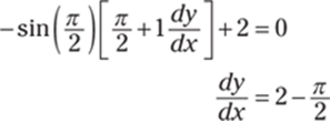
The tangent line has a slope of ![]() and passes through
and passes through ![]() , so its equation is
, so its equation is 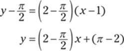
422. y = 1
You know a point on the tangent line, so you just need to find the slope. Begin by simplifying the left side of the equation. 
Next, find the derivative:
Use the values x = 0 and y = 1 and solve for the slope ![]() :
: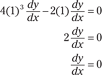
The tangent line has a slope of 0 and passes through (0, 1), so its equation is
423. ![]()
Use the formula for the differential, dy = f '(x) dx:

So for the given values, x = 3 and ![]() , find dy:
, find dy:

424. ![]()
Use the formula for the differential, dy = f '(x) dx:
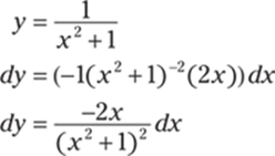
So for the given values, x = 1 and dx = –0.1, find dy:
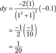
425. ![]()
Use the formula for the differential, dy = f '(x) dx:

So for the given values, ![]() and dx = 0.02, find dy:
and dx = 0.02, find dy:
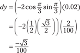
426. L(x) = 6x – 3
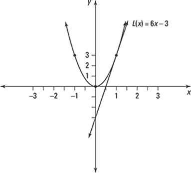
Finding the linearization L(x) is the same as finding the equation of the tangent line. First find a point on the line by entering the value of a in the function. For the given value of a, the corresponding y value is
![]()
Next, find the derivative of the function to get the slope of the line:

Using the point-slope formula with the slope m = 6 and the point (1, 3) gives you
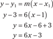
Replace y with L(x) to get the solution: L(x) = 6x – 3.
427. ![]()
Finding the linearization L(x) is the same as finding the equation of the tangent line. First find a point on the line by entering the value of a in the function. For the given value of a, the corresponding y value is
![]()
Next, find the derivative of the function to get the slope of the line:

Using the point-slope formula with the slope m = –1 and the point ![]() gives you
gives you
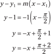
Replace y with L(x) to get the solution: ![]() .
.
428. 
Finding the linearization L(x) is the same as finding the equation of the tangent line. First find a point on the line by entering the value of a in the function. For the given value of a, the corresponding y value is
![]()
Next, find the derivative of the function to get the slope of the line:

Using the point-slope formula with the slope  and the point (2, 61/3) gives you
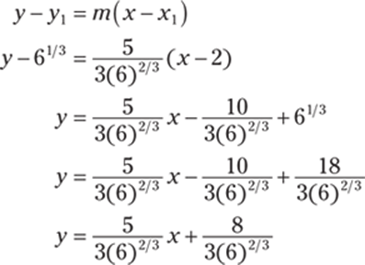
Replace y with L(x) to get the solution:
 .
.
429. 3.987
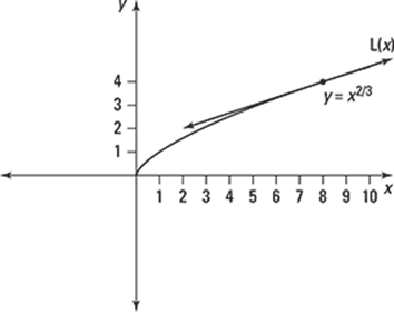
To estimate the value, you can find a linearization by using f (x) = x2/3 and a = 8 and then substitute 7.96 into the linearization.
Find a point on the line by entering the value of a in the function. For the given value of a, the corresponding y value is
![]()
Next, find the derivative of the function to get the slope of the line:
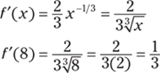
Using the point-slope formula with the slope ![]() and the point (8, 4) gives you
and the point (8, 4) gives you
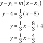
Replacing y with L(x) gives you the linearization
![]() .
.
Finally, substitute in the value x = 7.96 to find the estimate:
![]()
430. ![]()
To estimate the value, you can find a linearization by using ![]() and a = 100 and then substitute 102 into the linearization.
and a = 100 and then substitute 102 into the linearization.
Find a point on the line by entering the value of a in the function. For the given value of a, the corresponding y value is
![]()
Next, find the derivative of the function to get the slope of the line:
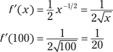
Using the point-slope formula with slope ![]() and point (100, 10) gives you
and point (100, 10) gives you
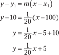
Replacing y with L(x) gives you the linearization ![]() .
.
Finally, substitute in the value x = 102 to find the estimate:

431. ![]()
To estimate the value of tan 46°, you can find a linearization using f (x) = tan x and ![]() and then substitute the value
and then substitute the value ![]() into the linearization.
into the linearization.
Find a point on the line by entering the value of a in the function. For the given value of a, the corresponding y value is
![]()
Next, find the derivative of the function to get the slope of the line:

Using the point-slope formula with slope m = 2 and point ![]() gives you
gives you
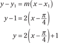
Replacing y with L(x) gives you the linearization ![]() .
.
Finally, substitute in the value of x = ![]() radians (that is, 46°) to find the estimate of tan 46°:
radians (that is, 46°) to find the estimate of tan 46°:
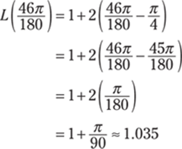
432. ![]()
The volume of a sphere is ![]() . To find the rate of expansion, take the derivative of each side with respect to time:
. To find the rate of expansion, take the derivative of each side with respect to time:
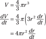
433. 8π m2/s
The area of a circle is A = πr2. To find the rate of increase, take the derivative of each side with respect to time:
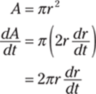
The circle increases at a rate of ![]() meter per second, so when radius r = 4 meters, the area increases at the following rate:
meter per second, so when radius r = 4 meters, the area increases at the following rate:
![]()
434. 508
Take the derivative of both sides with respect to t:

Then substitute in the given values, x = 3 and ![]() :
:
![]()
435. ![]()
Take the derivative of both sides with respect to t:

To find the value of z, enter x = 4 and y = 1 in the original equation:

Then substitute in the given values along with the value of z and solve for ![]() :
:
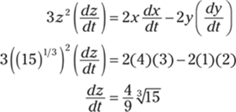
436. 2.49 m2/s

To find the area of the triangle, you need the base and the height. If you let the length of the base equal 8 meters, then one side of the triangle equals 6 meters. Therefore, if the height equals h, then ![]() so that
so that ![]() .
.
Because the area of a triangle is ![]() , you can write the area as
, you can write the area as

This equation now involves ![]() , so you can take the derivative of both sides with respect to t to get the rate of increase:
, so you can take the derivative of both sides with respect to t to get the rate of increase:
![]()
Substitute in the given values, ![]() and
and ![]() radians/second, and simplify:
radians/second, and simplify:
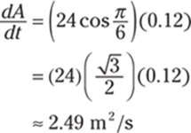
When the angle between the sides is ![]() , the area is increasing at a rate of about 2.49 square meters per second.
, the area is increasing at a rate of about 2.49 square meters per second.
437. ![]() rad/s
rad/s
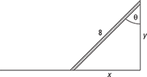
The problem tells you how quickly the bottom of the ladder slides away from the wall ![]() , so first write an expression for x, the distance from the wall. Assuming that the ground and wall meet at a right angle, you can write
, so first write an expression for x, the distance from the wall. Assuming that the ground and wall meet at a right angle, you can write

Taking the derivative with respect to time, t, gives you the rate at which the angle is changing:
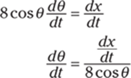
Substitute in the given information, where ![]() and
and ![]() feet per second:
feet per second:

When the angle is ![]() , the angle is increasing at a rate of
, the angle is increasing at a rate of ![]() radians per second.
radians per second.
438. 72 cm2/min
The area of a triangle is ![]() , and the problem tells you how quickly the base and height are changing. To find the rate of the change in area, take the derivative of both sides of the equation with respect to time, t:
, and the problem tells you how quickly the base and height are changing. To find the rate of the change in area, take the derivative of both sides of the equation with respect to time, t:
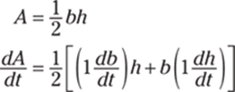
Note that you have to use the product rule to find the derivative of the right side of the equation.
Substitute in the given information, ![]() centimeters per minute, h = 32 centimeters, b = 20 centimeters, and
centimeters per minute, h = 32 centimeters, b = 20 centimeters, and ![]() centimeters per minute:
centimeters per minute:

439. 13.56 km/h

Let x be the distance sailed by Ship A and let y be the distance sailed by Ship B. Using the Pythagorean theorem, the distance between the ships is
![]()
From the given information, you have ![]() kilometers per hour and
kilometers per hour and ![]() kilometers per hour. Taking the derivative of both sides of the equation with respect to time gives you
kilometers per hour. Taking the derivative of both sides of the equation with respect to time gives you
![]()
Notice that after 3 hours have elapsed, x = 60 and y = 105. Therefore, using the Pythagorean theorem, you can deduce that ![]() kilometers.
kilometers.
Substitute in all these values and solve for ![]() :
:

At 3 p.m., the ships are moving apart at a rate of about 13.56 kilometers per hour.
440. 4.83 cm/s
From the Pythagorean theorem, the distance from the origin is D2 = x2 + y2. Using the particle's path, ![]() , you get
, you get

Taking the derivative of both sides with respect to time gives you
![]()
From the given values x = 8 centimeters and y = 3 centimeters, you find that the distance from the origin is ![]() centimeters. Use these values along with
centimeters. Use these values along with ![]() centimeters per second and solve for
centimeters per second and solve for ![]() :
:

441. 2.95 mi/h
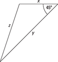
Let x be the distance that the person who is walking west has traveled, let y be the distance that the person traveling southwest has traveled, and let z be the distance between them.
Use the law of cosines to relate x, y, and z:

Take the derivative of both sides of the equation with respect to time:

After 40 minutes, or ![]() hour,
hour, ![]() and
and ![]() . Using the initial equation, you find that z ≈ 1.96 miles at this time. Substitute these values into the derivative and solve for
. Using the initial equation, you find that z ≈ 1.96 miles at this time. Substitute these values into the derivative and solve for ![]() :
:

After 40 minutes, the distance between these people is increasing at a rate of about 2.95 miles per hour.
442. ![]()

The water in the trough has a volume of ![]() . As the water level rises, the base and height of the triangle shapes increase. By similar triangles, you have
. As the water level rises, the base and height of the triangle shapes increase. By similar triangles, you have ![]() so that
so that ![]() . Therefore, the volume is
. Therefore, the volume is
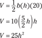
Taking the derivative with respect to time gives you
![]()
Use h = 1 foot and ![]() cubic feet per minute to find how quickly the water level is rising:
cubic feet per minute to find how quickly the water level is rising:
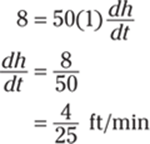
When the water is 1 foot deep, the water level is rising at a rate of ![]() feet per minute.
feet per minute.
443. 698.86 km/h
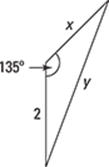
Let x be the distance that the jet travels, and let y be the distance between the jet and the radar station.
Use the law of cosines to relate x and y:
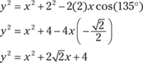
Taking the derivative of both sides of the equation with respect to time gives you
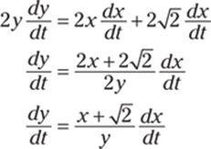
After 2 minutes, the jet has traveled ![]() kilometers, so the distance from the radar station is
kilometers, so the distance from the radar station is

Enter the value of y in the ![]() equation and solve:
equation and solve:

After 2 minutes, the jet is moving away from the radar station at a rate of about 698.86 kilometers per hour.
444. ![]()
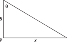
Let x be the distance from the Point P to the spot on the shore where the light is shining. From the diagram, you have ![]() , or
, or ![]() . Taking the derivative of both sides of the equation with respect to time gives you
. Taking the derivative of both sides of the equation with respect to time gives you
![]()
When x = 2, ![]() . Using a trigonometric identity, you have
. Using a trigonometric identity, you have

From the given information, you know that ![]() revolutions per minute. Because 2π radians are in one revolution, you can convert as follows:
revolutions per minute. Because 2π radians are in one revolution, you can convert as follows: ![]() radians per minute:
radians per minute:
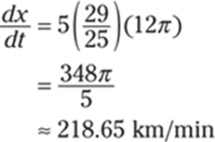
445. ![]()
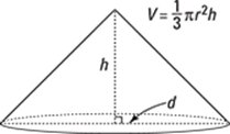
The volume of a cone is ![]() . The problem tells you that
. The problem tells you that ![]() cubic feet per minute and that d = 2h. Because the diameter is twice the radius, you have 2r = d = 2h so that r = h; therefore, the volume becomes
cubic feet per minute and that d = 2h. Because the diameter is twice the radius, you have 2r = d = 2h so that r = h; therefore, the volume becomes

Take the derivative with respect to time:
![]()
Substitute in the given information and solve for ![]() :
:
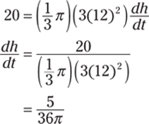
When the pile is 12 feet high, the height of the pile is increasing at a rate of ![]() (about 0.04) feet per minute.
(about 0.04) feet per minute.
446. no absolute maximum; absolute minimum: y = –1; no local maxima; local minimum: (1, –1)
There's no absolute maximum because the graph doesn't attain a largest y value. There are also no local maxima. The absolute minimum is y = –1. The point (1, –1) is a local minimum.
447. absolute maximum: y = 4; absolute minimum: y = 0; local maximum: (5, 4); local minima: (1, 0), (7, 2)
The absolute maximum value is 4, which the graph attains at the point (5, 4). The absolute minimum is 0, which is attained at the point (1, 0). The point (5, 4) also corresponds to a local maximum, and the local minima occur at (1, 0) and (7, 2).
448. absolute maximum: y = 3; no absolute minimum; local maxima: (3, 3), (5, 3); local minimum: (4, 1)
The absolute maximum value is 3, which the graph attains at the points (3, 3) and (5, 3). The function approaches the x-axis but doesn't cross or touch it, so there's no absolute minimum. The points (3, 3) and (5, 3) also correspond to local maxima, and the local minimum occurs at (4, 1).
449. no maxima or minima
The graph has no absolute maximum or minimum because the graph approaches ∞ on the left and –∞ on the right. Likewise, there are no local maxima or minima because (2, 1) and (5, 3) are points of discontinuity.
450. I and II
Because Point A satisfies the definition of both a local maximum and a local minimum, it's both. The graph decreases to negative infinity on the left side, so Point A is not an absolute minimum.
451. absolute maximum: 5; absolute minimum: –7
Begin by finding the derivative of the function; then find any critical numbers on the given interval by determining where the derivative equals zero or is undefined. Note that by finding critical numbers, you're finding potential turning points or cusp points of the graph.
The derivative of f (x) = 3x2 – 12x + 5 is

Setting the derivative equal to zero and solving gives you the only critical number, x = 2. Next, substitute the endpoints of the interval and the critical number into the original function and pick the largest and smallest values:

Therefore, the absolute maximum is 5, and the absolute minimum is –7.
452. absolute maximum: 67; absolute minimum: 3
Begin by finding the derivative of the function; then find any critical numbers on the given interval. The derivative of f (x) = x4 – 2x2 + 4 is

Setting the derivative equal to zero and solving gives you the critical numbers x = 0 and x = ±1, all of which fall within the given interval. Next, substitute the endpoints of the interval along with the critical numbers into the original function and pick the largest and smallest values:
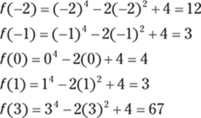
Therefore, the absolute maximum is 67, and the absolute minimum is 3.
453. absolute maximum: ![]() ; absolute minimum: 0
; absolute minimum: 0
Begin by finding the derivative of the function; then find any critical numbers on the given interval. The derivative of ![]() is
is

Next, find the critical numbers by setting the numerator equal to zero and solving for x (note that the denominator will never be zero):

Only x = 1 is in the given interval, so don't use x = –1. Next, substitute the endpoints of the interval along with the critical number into the original function and pick the largest and smallest values:

Therefore, the absolute maximum is ![]() , and the absolute minimum is 0.
, and the absolute minimum is 0.
454. absolute maximum: 2; absolute minimum: ![]()
Begin by finding the derivative of the function; then find any critical numbers on the given interval. The derivative of ![]() is
is
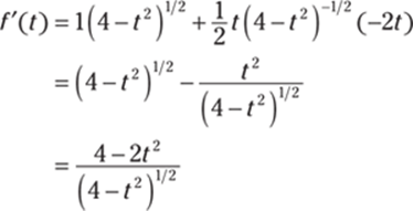
Next, find any critical numbers of the function by setting the numerator and denominator of the derivative equal to zero and solving for t.
From the numerator of the derivative, you have 4 – 2t2 = 0 so that 4 = 2t2, or 2 = t2, which has the solutions ![]() . From the denominator, you have 4 – t2 = 0, or 4 = t2, which has the solutions t = ±2.
. From the denominator, you have 4 – t2 = 0, or 4 = t2, which has the solutions t = ±2.
Substitute the endpoints along with the critical points that fall within the interval into the original function and pick the largest and smallest values:
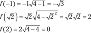
Therefore, the absolute maximum is 2, and the absolute minimum is ![]() .
.
455. absolute maximum: π + 2; absolute minimum: ![]()
Begin by finding the derivative of the function; then find any critical numbers on the given interval. The derivative of f (x) = x – 2 cos x is
![]()
Setting the derivative equal to zero in order to find the critical numbers gives you 1+ 2 sin x = 0, or ![]() , which has the solutions
, which has the solutions ![]() and
and ![]() in the given interval of [–π, π].
in the given interval of [–π, π].
Substitute these critical numbers along with the endpoints of the interval into the original function and pick the largest and smallest values:
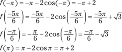
Therefore, the absolute maximum is π + 2, and the absolute minimum is ![]() .
.
456. increasing on (–∞, –2) and (2, ∞); decreasing on (–2, 2)
Begin by finding the derivative of the function; then find any critical numbers on the given interval by determining where the derivative equals zero or is undefined. Note that by finding critical numbers, you're finding potential turning points or cusp points of the graph.
The derivative of the function f (x) = 2x3 – 24x + 1 is

Setting the derivative equal to zero in order to find the critical points gives you x2 – 4 = 0, or x2 = 4, so that x = ±2.
To determine where the function is increasing or decreasing, substitute a test point inside each interval into the derivative to see whether the derivative is positive or negative.
To test (–∞, –2), you can use x = –3. In that case, f '(–3) = 6(–3)2 – 24 = 30. The derivative is positive, so the function is increasing on (–∞, –2). Proceed in a similar manner for the intervals (–2, 2) and (2, ∞). When x = 0, you have f '(0) = 6(0)2 – 24 = –24, so the function is decreasing on (–2, 2). And if x = 3, then f '(3) = 6(3)2 – 24 = 30, so the function is increasing on (2, ∞).
457. increasing on (–2, ∞); decreasing on (–3, –2)
Begin by finding the derivative of the function. The derivative of ![]() is
is
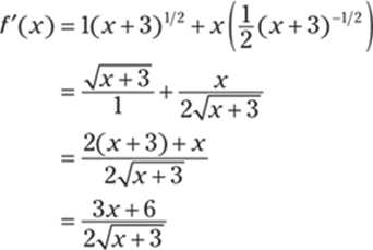
Next, find any critical numbers that fall inside the interval (–3, ∞) by setting the derivative equal to zero and solving for x. (You only need to set the numerator equal to zero, because the denominator will never equal zero.) This gives you 3x + 6 = 0, or x = –2.
Next, pick a value in (–3, –2) and determine whether the derivative is positive or negative. So if x = –2.5, then  ; therefore, the function is decreasing on (–3, –2). Likewise, you can show that f '(x) > 0 on (–2, ∞), which means that f (x) is increasing on (–2, ∞).
458. increasing on ![]() ,
, ![]() ; decreasing on
; decreasing on ![]() ,
, ![]() ,
, ![]()
Begin by finding the derivative of the function. The derivative of f (x) = cos2 x – sin x is
![]()
Next, find any critical numbers that fall inside the specified interval by setting the derivative equal to zero and solving: –2 cos x sin x = 0, or (–cos x)(2 sin x + 1) = 0. Solving –cos x = 0 gives you the solutions ![]() and
and ![]() , and solving 2 sin + 1 = 0 gives you
, and solving 2 sin + 1 = 0 gives you ![]() , which has the solutions
, which has the solutions ![]() and
and ![]() .
.
To determine where the original function is increasing or decreasing, substitute a test point from inside each interval into the derivative to see whether the derivative is positive or negative. So for the interval ![]() , you can use
, you can use ![]() . In that case,
. In that case, ![]() , so the function is decreasing on
, so the function is decreasing on ![]() . Proceeding in a similar manner, you can show that for a point inside the interval
. Proceeding in a similar manner, you can show that for a point inside the interval ![]() , f ' > 0; that for a point inside the interval
, f ' > 0; that for a point inside the interval ![]() , f '> 0; that for a point inside
, f '> 0; that for a point inside ![]() , f ' > 0; and that for a point inside
, f ' > 0; and that for a point inside ![]() , f ' > 0. Therefore, f (x) is increasing on
, f ' > 0. Therefore, f (x) is increasing on ![]() and
and ![]() , and f (x) is decreasing on
, and f (x) is decreasing on ![]() ,
, ![]() , and
, and ![]() .
.
459. increasing on ![]() ,
, ![]() ; decreasing on
; decreasing on ![]() ,
, ![]()
Begin by finding the derivative of the function. The derivative of f (x) = 2 cos x – cos 2x is

Now find the critical numbers by setting each factor equal to zero and solving for x. The equation sin x = 0 gives you the solutions x = 0, x = π, and x = 2π. Solving 2 cos x – 1 = 0 gives you ![]() , which has solutions
, which has solutions ![]() and
and ![]() .
.
To determine whether the function is increasing or decreasing on ![]() , pick a point in the interval and substitute it into the derivative. So if you use
, pick a point in the interval and substitute it into the derivative. So if you use ![]() , then you have
, then you have ![]() , so the function is increasing on
, so the function is increasing on ![]() . Likewise, if you use the point
. Likewise, if you use the point ![]() in the interval
in the interval ![]() , you have
, you have ![]() . If you use
. If you use ![]() in the interval
in the interval ![]() , then
, then ![]() . And if you use
. And if you use ![]() in the interval
in the interval ![]() , you have
, you have ![]() . Therefore, f (x) is increasing on the intervals
. Therefore, f (x) is increasing on the intervals ![]() and
and ![]() , and f (x) is decreasing on the intervals
, and f (x) is decreasing on the intervals ![]() and
and ![]() .
.
460. increasing on (0, 1); decreasing on (1, ∞)
Begin by finding the derivative of the function. The derivative of f (x) = 4 ln x – 2x2 is
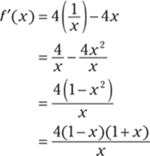
Now find the critical numbers. Setting the numerator equal to zero gives you (1 – x)(1 + x) = 0 so that x = 1 or –1. Setting the denominator of the derivative equal to zero gives you x = 0. Notice that neither x = 0 nor x = –1 is in the domain of the original function.
To determine whether the function is increasing or decreasing on (0, 1), take a point in the interval and substitute it into the derivative. If ![]() , then
, then 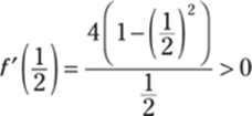 , so the function is increasing on (0, 1). Likewise, if you use x = 2, then
 ![]() , so the function is decreasing on (1, ∞).
, so the function is decreasing on (1, ∞).
461. local maximum at (–1, 7); local minimum at (2, –20)
Begin by finding the derivative of the function f (x) = 2x3 – 3x2 – 12x:
![]()
Then set this derivative equal to zero and solve for x to find the critical numbers:
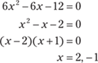
Next, determine whether the function is increasing or decreasing on the intervals (–∞, –1), (–1, 2), and (2, ∞) by picking a point inside each interval and substituting it into the derivative. Using the values x = –2, x = 0, and x = 3 gives you

Therefore, f (x) is increasing on (–∞, –1), decreasing on (–1, 2), and increasing again on (2, ∞). That means there's a local maximum at x = –1 and a local minimum at x = 2.
Now enter these values in the original function to find the coordinates of the local maximum and minimum. Because f (–1) = 2(–1)3 – 3(–1)2 – 12(–1) = 7, the local maximum occurs at (–1, 7). Because f (2) = 2(2)3 – 3(2)2 – 12(2) = –20, the local minimum occurs at (2, –20).
462. no local maxima; local minimum at (16, –16)
Begin by finding the derivative of the function ![]() :
:
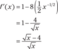
Then find the critical numbers. Setting the numerator equal to zero gives you ![]() so that
so that ![]() , or x = 16. Setting the denominator equal to zero gives you x = 0. Next, determine whether the function is increasing or decreasing on the intervals (0, 16) and (16, ∞) by taking a point in each interval and substituting it into the derivative. So if x = 1, you have
, or x = 16. Setting the denominator equal to zero gives you x = 0. Next, determine whether the function is increasing or decreasing on the intervals (0, 16) and (16, ∞) by taking a point in each interval and substituting it into the derivative. So if x = 1, you have ![]() so that f (x) is decreasing on (0, 16). And if x = 25, you have
so that f (x) is decreasing on (0, 16). And if x = 25, you have  , so f (x) is increasing on (16, ∞). Therefore, the function has a local minimum at x = 16. Finish by finding the coordinates:
 ![]() , so the local minimum is at (16, –16).
, so the local minimum is at (16, –16).
463. local maximum at (64, 32); local minimum at (0, 0)
Begin by finding the derivative of the function f (x) = 6x2/3 – x:
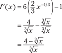
Then find the critical numbers. Setting the numerator equal to zero gives you ![]() so that 4 = x1/3, or 64 = x. Setting the denominator equal to zero gives you x = 0 as a solution.
so that 4 = x1/3, or 64 = x. Setting the denominator equal to zero gives you x = 0 as a solution.
Next, determine whether the function is increasing or decreasing on the intervals (–∞, 0), (0, 64), and (64, ∞) by taking a point in each interval and substituting it into the derivative. Using the test points x = –1, x = 1, and x = 125 gives you the following:
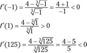
Therefore, f (x) is decreasing on (–∞, 0), increasing on (0, 64), and decreasing on (64, ∞). That means f (x) has a local minimum at x = 0; f (0) = 0, so a local minimum occurs at (0, 0). Also, f (x) has a local maximum at x = 64; f (64) = 6(64)2/3 – 64 = 32, so the local maximum occurs at (64, 32).
464. local maximum at  ; local minimum at
Begin by finding the derivative of the function f (x) = 2 sin x – sin 2x:
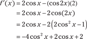
Next, find the critical numbers by setting the derivative equal to zero:

Setting the first factor equal to zero gives you ![]() , which has the solutions
, which has the solutions ![]() and
and ![]() . Setting the second factor equal to zero gives you
. Setting the second factor equal to zero gives you ![]() , which has the solutions x = 0 and 2π.
, which has the solutions x = 0 and 2π.
Next, determine whether the function is increasing or decreasing on the intervals  ,
, ![]() , and
, and ![]() by taking a point inside each interval and substituting it into the derivative to see whether it's positive or negative. Using the points
by taking a point inside each interval and substituting it into the derivative to see whether it's positive or negative. Using the points ![]() , π, and
, π, and ![]() gives you
gives you


So f (x) has a local maximum when ![]() because the function changes from increasing to decreasing at this value, and f (x) has a local minimum when
because the function changes from increasing to decreasing at this value, and f (x) has a local minimum when ![]() because the function changes from decreasing to increasing at this value.
because the function changes from decreasing to increasing at this value.
To find the points on the original function, substitute in these values. If ![]() , then
, then
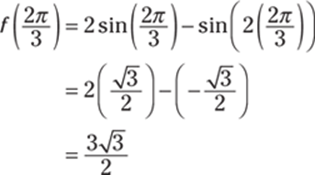
So the local maximum occurs at  . If
. If ![]() , then
, then
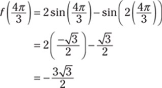
Therefore, the local minimum occurs at  .
.
465. local maxima at ![]() ,
, ![]() ; local minima at
; local minima at ![]() ,
, ![]()
Begin by finding the derivative of the function f (x) = x + 2 cos x:
![]()
Next, find the critical numbers by setting the function equal to zero and solving for x on the given interval:
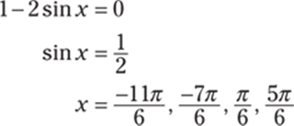
Then determine whether the function is increasing or decreasing on the intervals ![]() ,
, ![]() ,
, ![]() ,
, ![]() , and
, and ![]() by taking a point inside each interval and substituting it into the derivative. Using the value x = –6.27, which is slightly larger than –2π, gives you f '(–6.27) ≈ f '(–2π) = 1 > 0. Likewise, using the points
by taking a point inside each interval and substituting it into the derivative. Using the value x = –6.27, which is slightly larger than –2π, gives you f '(–6.27) ≈ f '(–2π) = 1 > 0. Likewise, using the points ![]() , 0,
, 0, ![]() , and
, and ![]() from each of the remaining four intervals gives you the following:
from each of the remaining four intervals gives you the following:
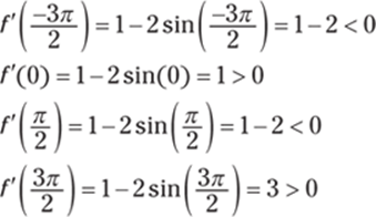
Therefore, the function has local maxima when ![]() and
and ![]() and local minima when
and local minima when ![]() and
and ![]() . To find the points on the original function, substitute these x values into the original function:
. To find the points on the original function, substitute these x values into the original function:
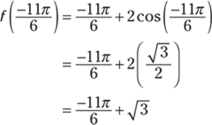
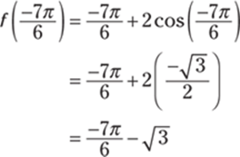
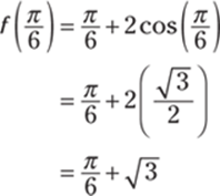
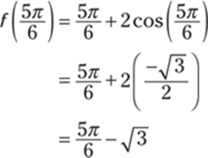
Therefore, the local maxima are ![]() and
and ![]() , and the local minima are
, and the local minima are ![]() and
and ![]() .
.
466. concave up on (1, ∞); concave down on (–∞, 1)
To determine concavity, examine the second derivative. Because a derivative measures a “rate of change” and the first derivative of a function gives the slopes of tangent lines, the derivative of the derivative (the second derivative) measures the rate of change of the slopes of the tangent lines. If the second derivative is positive on an interval, the slopes of the tangent lines are increasing, so the function is bending upward, or is concave up. Likewise, if the second derivative is negative on an interval, the slopes of the tangent lines are decreasing, so the function is bending downward, or is concave down.
Begin by finding the first and second derivatives of the function f (x) = x3 – 3x2 + 4:

Setting the second derivative equal to zero gives you 6x – 6 = 0 so that x = 1.
To determine the concavity on the intervals (–∞, 1) and (1, ∞), pick a point from each interval and substitute it into the second derivative to see whether it's positive or negative. Using the values x = 0 and x = 2, you have f "(0) = 6(0) – 6 > 0 and f "(2) = 6(2) – 6 > 0. Therefore, f (x) is concave up on the interval (1, ∞) and concave down on the interval (–∞, 1).
467. concave up nowhere; concave down on (–∞, 0), (0, ∞)
Begin by finding the first and second derivatives of the function f (x) = 9x2/3 – x:

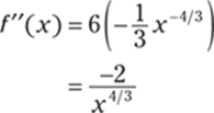
Next, set the denominator of the second derivative equal to zero to get x4/3 = 0 so that x = 0.
To determine the concavity on the intervals (–∞, 0) and (0, ∞), pick a point from each interval and substitute it into the second derivative to see whether it's positive or negative. Using the values x = –1 and x = 1, you have the following:
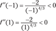
Therefore, the f (x) is concave down on the intervals (–∞, 0) and (0, ∞).
468. concave up on (–∞, 0), ![]() ; concave down on
; concave down on ![]()
Begin by finding the first derivative of the function f (x) = x1/3(x + 1) = x4/3 + x1/3:
![]()
Next, use the power rule to find the second derivative:
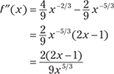
Then find where the second derivative is equal to zero or undefined. Setting the numerator equal to zero gives you 2x – 1 = 0 so that ![]() , and setting the denominator equal to zero gives you 9x5/3 = 0 so that x = 0.
, and setting the denominator equal to zero gives you 9x5/3 = 0 so that x = 0.
To determine the concavity on the intervals (–∞, 0), ![]() , and
, and ![]() , pick a point from each interval and substitute it into the second derivative to see whether it's positive or negative. Using the values x = –1,
, pick a point from each interval and substitute it into the second derivative to see whether it's positive or negative. Using the values x = –1, ![]() , and x = 1 gives you the following:
, and x = 1 gives you the following:
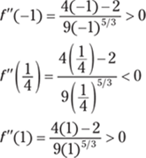
Therefore, f (x) is concave up on the intervals (–∞, 0) and ![]() , and f (x) is concave down on the interval
, and f (x) is concave down on the interval ![]() .
.
469. concave up on (–∞, –2),  , (2, ∞); concave down on
  ,
, 
Begin by finding the first and second derivatives of the function f (x) = (x2 – 4)3:

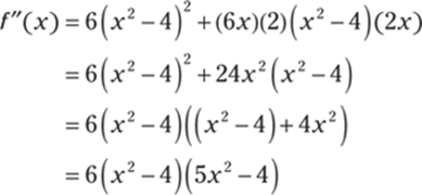
Next, set each factor in the second derivative equal to zero and solve for x: x2 – 4 = 0 gives you the solutions x = 2 and x = –2, and 5x2 – 4 = 0, or ![]() , has the solutions
, has the solutions  and
and  .
.
To determine the concavity on the intervals (–∞, –2),  ,
,  ,
,  , and (2, ∞), pick a point from each interval and substitute it into the second derivative to see whether it's positive or negative. Using the values x = –3, x = –1, x = 0, x = 1, and x = 3, you have the following:
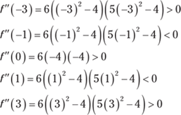
Therefore, f (x) is concave up on the intervals (–∞, –2),  , and (2, ∞), and f (x) is concave down on the intervals
  and
and  .
.
470. concave up on ![]() ,
, ![]() ; concave down on the intervals (0, 0.253),
; concave down on the intervals (0, 0.253), ![]() ,
, ![]()
Begin by finding the first and second derivatives of the function f (x) = 2 cos x – sin(2x):

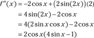
Next, set each factor of the second derivative equal to zero and solve: cos x = 0 has the solutions ![]() and
and ![]() , and 4 sin x – 1 = 0, or
, and 4 sin x – 1 = 0, or ![]() , has the solutions
, has the solutions ![]() and x = π – 0.253.
and x = π – 0.253.
To determine the concavity on the intervals (0, 0.25), ![]() ,
, ![]() ,
, ![]() , and
, and ![]() , pick a point from each interval and substitute it into the second derivative to see whether it's positive or negative. Using the values x = 0.1,
, pick a point from each interval and substitute it into the second derivative to see whether it's positive or negative. Using the values x = 0.1, ![]() ,
, ![]() , x = π, and
, x = π, and ![]() gives you the following:
gives you the following:
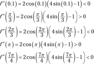
Therefore, f (x) is concave up on the intervals ![]() and
and ![]() , and f (x) is concave down on the intervals (0, 0.253),
, and f (x) is concave down on the intervals (0, 0.253), ![]() , and
, and ![]() .
.
471. no inflection points
Inflection points are points where the function changes concavity. To determine concavity, examine the second derivative. Because a derivative measures a “rate of change” and the first derivative of a function gives the slopes of tangent lines, the derivative of the derivative (the second derivative) measures the rate of change of the slopes of the tangent lines. If the second derivative is positive on an interval, the slopes of the tangent lines are increasing, so the function is bending upward, or is concave up. Likewise, if the second derivative is negative on an interval, the slopes of the tangent lines are decreasing, so the function is bending downward, or is concave down.
Begin by finding the first and second derivatives of the function ![]() . The first derivative is
. The first derivative is
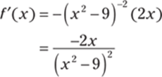
Now find the second derivative:
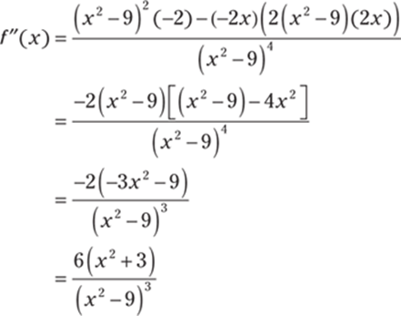
Notice that the numerator of the second derivative never equals zero and that the denominator equals zero when x = ±3; however, x = ±3 isn't in the domain of the original function. Therefore, there can be no inflection points.
472. ![]()
Begin by finding the first and second derivatives of the function f (x) = 2x3 + x2. The first derivative is
![]()
And the second derivative is
![]()
Setting the second derivative equal to zero gives you 12x + 2 = 0, which has the solution ![]() .
.
To determine the concavity on the intervals ![]() and
and ![]() , pick a point from each interval and substitute it into the second derivative to see whether it's positive or negative. Using the values x = –1 and x = 0 gives you the following:
, pick a point from each interval and substitute it into the second derivative to see whether it's positive or negative. Using the values x = –1 and x = 0 gives you the following:

Therefore, the function is concave down on the interval ![]() and concave up on the interval
and concave up on the interval ![]() , so
, so ![]() is an inflection point. The corresponding y value on f (x) is
is an inflection point. The corresponding y value on f (x) is
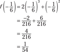
Therefore, the inflection point is ![]() .
.
473. no inflection points
Being by finding the first and second derivatives of the function ![]() . The first derivative is
. The first derivative is
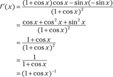
And the second derivative is

Next, find where the second derivative is equal to zero or undefined. Setting the numerator equal to zero gives you sin x = 0, which has solutions x = 0, x = π, and x = 2π. Setting the denominator equal to zero gives you 1 + cos x = 0, or cos x = –1, which has the solution x = π.
To determine the concavity on the intervals (0, π) and (π, 2π), pick a point from each interval and substitute it into the second derivative to see whether it's positive or negative. Using the values ![]() and
and ![]() gives you the following:
gives you the following:
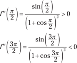
However, note that at x = π, the original function is undefined, so there are no inflection points. In fact, if you noticed this at the beginning, there's really no need to determine the concavity on the intervals!
474. (π, 0)
Begin by finding the first and second derivatives of the function f (x) = 3 sin x – sin3 x. The first derivative is
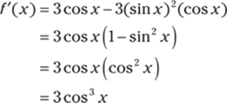
And the second derivative is

Next, find where the second derivative is equal to zero by setting each factor equal to zero: cos x has the solutions ![]() and
and ![]() , and sin x = 0 has the solutions x = 0, x = π, and x = 2π.
, and sin x = 0 has the solutions x = 0, x = π, and x = 2π.
To determine the concavity on the intervals ![]() ,
, ![]() ,
, ![]() , and
, and ![]() , pick a point from each interval and substitute it into the second derivative to see whether it's positive or negative. Using the values
, pick a point from each interval and substitute it into the second derivative to see whether it's positive or negative. Using the values ![]() ,
, ![]() ,
, ![]() , and
, and ![]() , you have the following:
, you have the following:
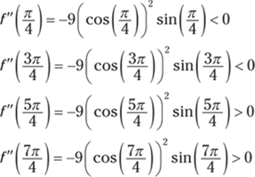
Therefore, the concavity changes when x = π. The corresponding y value on f (x) is f (π) = 3 sin π – (sin π)3 = 0, so the inflection point is (π, 0).
475. (–1, –6)
Begin by finding the first and second derivatives of the function f (x) = x5/3 – 5x2/3. The first derivative is

And the second derivative is
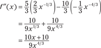
Next, find where the second derivative is equal to zero or undefined by setting the numerator and the denominator equal to zero. For the numerator, you have 10x + 10 = 0, which has the solution x = –1. For the denominator, you have 9x4/3 = 0, which has the solution x = 0.
To determine the concavity on the intervals (–∞, –1), (1, 0), and (0, ∞), pick a point from each interval and substitute it into the second derivative to see whether it's positive or negative. Using the values x = –2, ![]() , and x = 1 gives you
, and x = 1 gives you
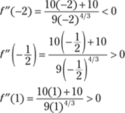
Because the concavity changes at x = –1, the original function has an inflection point there. The corresponding y value on f (x) is

Therefore, the inflection point is (–1, –6).
476. no local maxima; local minimum at (0, 1)
Begin by finding the first derivative of the function ![]() :
:
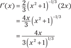
Next, find any critical numbers of the function. Setting the numerator of the derivative equal to zero gives you the solution x = 0. Note that no real values can make the denominator equal to zero.
Then find the second derivative:
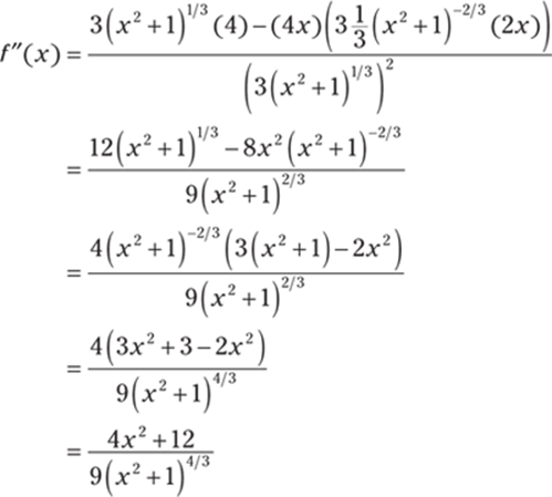
To see whether the original function is concave up or concave down at the critical number, substitute x = 0 into the second derivative:

The second derivative is positive, so the original function is concave up at the critical point; therefore, a local minimum is at x = 0. The corresponding y value on the original function is ![]() , so the local minimum is at (0, 1).
, so the local minimum is at (0, 1).
477. local maximum at (0, 1); local minima at ![]() ,
, ![]()
Begin by finding the first derivative of the function f (x) = x4 – 4x2 + 1:

Set the first derivative equal to zero and solve for x to find the critical numbers of f. The critical numbers are x = 0, ![]() , and
, and ![]() .
.
Next, find the second derivative:
![]()
Substitute each of the critical numbers into the second derivative to see whether the second derivative is positive or negative at those values:
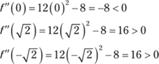
Therefore, the original function has a local maximum when x = 0 and local minima when ![]() and
and ![]() . The corresponding y values on the original function are
. The corresponding y values on the original function are ![]() , f (0) = 04 – 4(0)2 + 1 = 1, and
, f (0) = 04 – 4(0)2 + 1 = 1, and ![]() . Therefore, the local maximum occurs at (0, 1), and the local minima occur at
. Therefore, the local maximum occurs at (0, 1), and the local minima occur at ![]() and
and ![]() .
.
478. local maxima at  ,
,  ; local minimum at (0, 0)
Begin by finding the first derivative of the function f (x) = 2x2(1 – x2) = 2x2 – 2x4:

Set the first derivative equal to zero and solve for x to find the critical numbers. Solving 4x(1 – 2x2) = 0 gives you x = 0,  , and
, and  as the critical numbers.
Next, find the second derivative:
![]()
Substitute the critical numbers into the second derivative to see whether the second derivative is positive or negative at those values:
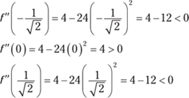
So the original function has local maxima when  and
and  and a local minimum when x = 0. Finding the corresponding y values on the original function gives you the following:
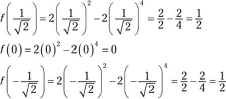
Therefore, the local maxima are at  and
and  , and the local minimum is at (0, 0).
479. local maximum at ![]() ; local minimum at
; local minimum at ![]()
Begin by finding the first derivative of the function ![]() :
:
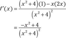
Then set the numerator and denominator of the first derivative equal to zero to find the critical numbers. Setting the numerator equal to zero gives you –x2 + 4 = 0, which has the solutions x = 2 and x = –2. Notice that the denominator of the derivative doesn't equal zero for any value of x.
Next, find the second derivative of the function:
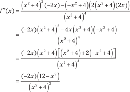
Substitute the critical numbers into the second derivative to see whether the second derivative is positive or negative at those values:
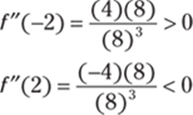
Because f (x) is concave up when x = –2 and concave down when x = 2, a local minimum occurs at x = –2, and a local maximum occurs when x = 2. Because ![]() and
and ![]() , the local minimum occurs at
, the local minimum occurs at ![]() , and the local maximum occurs at
, and the local maximum occurs at ![]() .
.
480. local maximum at ![]() ; local minimum at
; local minimum at ![]()
Begin by finding the first derivative of the function f (x) = 2 sin x – x:
![]()
Set the first derivative equal to zero to find the critical numbers. From the equation 2 cos x – 1 = 0, you get ![]() , so the critical numbers are
, so the critical numbers are ![]() and
and ![]() .
.
Next, find the second derivative:
![]()
Substitute the critical numbers into the second derivative to see whether the second derivative is positive or negative at these values:
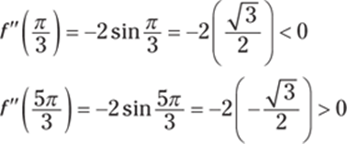
Because the function is concave down at ![]() , it has a local maximum there, and because the function is concave up at
, it has a local maximum there, and because the function is concave up at ![]() , it has a local minimum there. To find the corresponding y value on f (x), substitute the critical numbers into the original function:
, it has a local minimum there. To find the corresponding y value on f (x), substitute the critical numbers into the original function:
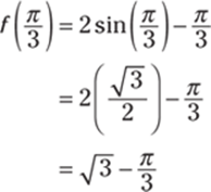
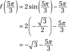
Therefore, the local maximum is at ![]() , and the local minimum is at
, and the local minimum is at ![]() .
.
481. ![]()
Recall Rolle's theorem: If f is a function that satisfies the following three hypotheses:
· f is continuous on the closed interval [a, b]
· f is differentiable on the open interval (a, b)
· f (a) = f (b)
then there is a number c in (a, b) such that f '(c) = 0.
Notice that the given function is differentiable everywhere (and therefore continuous everywhere) because it's a polynomial. Then verify that f (0) = f (6) so that Rolle's theorem can be applied:

Next, find the derivative of the function, set it equal to zero, and solve for c:

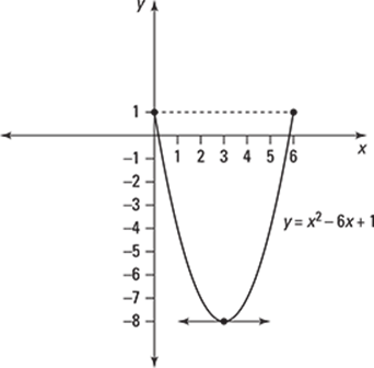
482. ![]()
Notice that the given function is differentiable on (–8, 0). Then verify that f (–8) = f (0) so that Rolle's theorem can be applied:

Next, find the derivative of the function, set it equal to zero, and solve. Here's the derivative:
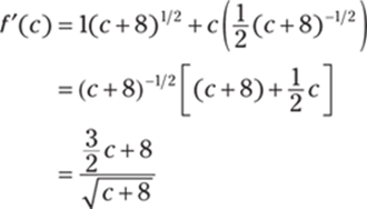
Setting the numerator equal to zero and solving for c gives you
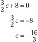
483. 0, ![]() , ±1
, ±1
Notice that the given function is differentiable everywhere. Then verify that f (–1) = f (1) so that Rolle's theorem can be applied:

Next, find the derivative of the function, set it equal to zero, and solve for c. Here's the derivative:

You need to find the solutions of sin(2πc) = 0 on the interval –1 ≤ c ≤ 1 so that –2π ≤ 2πc ≤ 2π. Notice that the solutions occur when 2πc = –2π, –π, 0, π, and 2π. Solving each of these equations for c gives you the solutions c = –1, ![]() , c = 0,
, c = 0, ![]() , and c = 1.
, and c = 1.
484. ![]()
Recall the mean value theorem: If f is a function that satisfies the following hypotheses:
· f is continuous on the closed interval [a, b]
· f is differentiable on the open interval (a, b)
then there is a number c in (a, b) such that ![]() .
.
Notice that the given function is differentiable everywhere, so you can apply the mean value theorem. Next, find the value of ![]() on the given interval:
on the given interval:
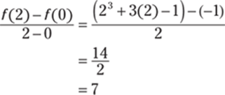
Now find the derivative of f (x) = x3 + 3x – 1, the given function, and set it equal to 7. The derivative is f ' = 3x2 + 3, so
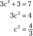
The negative root falls outside the given interval, so keeping only the positive root gives you the solution  .
.
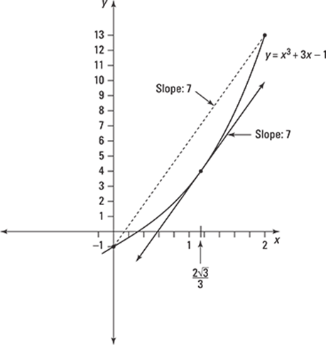
485. 
Notice that the given function is differentiable on (0, 1) and continuous on [0, 1], so you can apply the mean value theorem. Next, find the value of ![]() on the given interval:
on the given interval:
![]()
Now find the derivative of ![]() , the given function, and set it equal to 2. The derivative is
, the given function, and set it equal to 2. The derivative is ![]() , so you have
, so you have
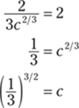
486. ![]()
Notice that the given function is differentiable everywhere, so you can apply the mean value theorem. Next, find the value of ![]() on the given interval:
on the given interval:
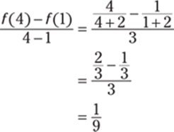
Now find the derivative of ![]() , the given function, and set it equal to
, the given function, and set it equal to ![]() . The derivative is
. The derivative is  , so you have

Keeping only the positive root, you have ![]() , which has the solution
, which has the solution ![]() . Note that the negative root would give you
. Note that the negative root would give you ![]() , which is outside of the interval.
, which is outside of the interval.
487. 24
By the mean value theorem, you have the following equation for some c on the interval [1, 5]:

Next, solve for f (5) using the fact that f (1) = 12 and f '(x) ≥ 3 (and so f '(c) ≥ 3):

488. 8 ≤ f (8) – f (4) ≤ 24
If 2 ≤ f '(x) ≤ 6, then by the mean value theorem, you have the following equation for some c in the interval [4, 8]:

Using 2 ≤ f '(x) ≤ 6, you can bound the value of 4f '(c) because 2 ≤ f '(c) ≤ 6:

Because f (8) – f (4) = 4f '(c), it follows that
![]()
489. ![]()
The given function ![]() is continuous and differentiable on the given interval. By the mean value theorem, there exists a number c in the interval [8, 9] such that
is continuous and differentiable on the given interval. By the mean value theorem, there exists a number c in the interval [8, 9] such that

But because ![]() , you have
, you have ![]() . Replacing
. Replacing ![]() in the equation
in the equation  gives you
![]()
Because ![]() , you have
, you have ![]() , so
, so
![]()
Notice also that f ' is decreasing (f " will be negative on the given interval), so the following is true:
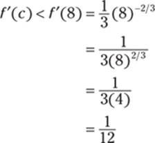
Because ![]() , you have
, you have ![]() . Therefore, it follows that
. Therefore, it follows that
![]()
490. velocity: 2; acceleration: 2
Begin by taking the derivative of the position function s(t) to find the velocity function:
![]()
Substituting in the value of t = 5, find the velocity:
![]()
Next, take the derivative of the velocity function to find the acceleration function:
![]()
Because the acceleration is a constant at t = 5, the acceleration is a(5) = 2.
491. velocity: 1; acceleration: –2
Begin by taking the derivative of the position function s(t) to find the velocity function:
![]()
Substituting in the value ![]() gives you the velocity:
gives you the velocity:
![]()
Next, take the derivative of the velocity function to find the acceleration function:
![]()
Substituting in the value of ![]() gives you the acceleration:
gives you the acceleration:

492. velocity: 0; acceleration: –1
Begin by taking the derivative of the position function s(t) to find the velocity function:
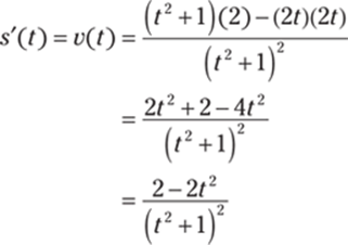
Substituting in the value t = 1 gives you the velocity:

Next, take the derivative of the velocity function to find the acceleration function:
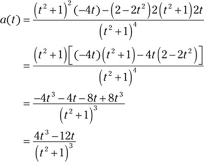
Substituting in the value of t = 1 gives you the acceleration:

493. compressing; speed: 8 ft/s
Begin by taking the derivative of the equation of motion to find the velocity function:
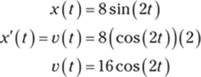
At ![]() , you have
, you have
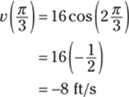
The velocity is negative, so the spring is compressing. Because the speed is the absolute value of the velocity, the speed is 8 feet per second.
494. maximum height: 25 ft; upward velocity: ![]() ft/s; downward velocity:
ft/s; downward velocity: ![]() ft/s
ft/s
One way to find the maximum height of the stone is to determine when the velocity of the stone is zero, because that's when the stone stops going upward and begins falling. (The stone follows a parabolic path, so you can also use the formula to find the vertex, but try the calculus way instead.)
Finding the derivative of the position function gives you the velocity function:

Set the velocity function equal to zero and solve for time t:
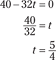
Substituting this time value into the position equation gives you

Therefore, the maximum height of the stone is 25 feet.
To answer the second part of the question, use algebra to find at what points in time the stone is at a height of 20 feet:

Using the quadratic formula with a = 4, b = –10, and c = 5, you get the solutions ![]() and
and ![]() . Substituting these values into the derivative gives you the velocity at these times:
. Substituting these values into the derivative gives you the velocity at these times:
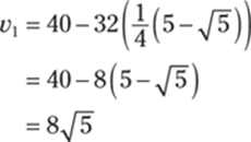
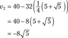
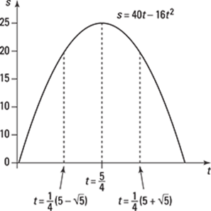
The velocities are approximately equal to 17.89 feet per second and –17.89 feet per second. The signs on the answers reflect that the stone is moving up at the first time and down at the second time.
495. maximum height: 6.25 ft; velocity on impact: –20 ft/s
One way to find the height of the stone is to determine when the velocity of the stone is zero, because that's when the stone stops going upward and begins falling. (The stone follows a parabolic path, so you can also use the formula to find the vertex, but try the calculus way instead.)
Finding the derivative of the position function gives you the velocity function:

Set the velocity function equal to zero and solve for time t:

Substitute in this value to find the height:

To find the velocity of the stone when it hits the ground, first determine when the stone hits the ground by setting the position equation equal to zero and solving for t:
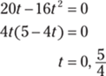
Because t = 0 corresponds to when the stone is first released, substitute ![]() into the velocity function to get the final velocity:
into the velocity function to get the final velocity:

496. downward on  ; upward on
Note that because the velocity is the rate of change in position with respect to time, you want to find when the velocity is positive and when the velocity is negative. Assume that when the velocity is positive, the particle is moving upward, and when the velocity is negative, the particle is moving downward.
Begin by taking the derivative of the position function to find the velocity function:

Set the velocity function equal to zero and solve for time t:

Use only the positive solution based on the given interval for t.
Now take a point from the interval  and a point from
  and substitute them into the velocity function to see whether the velocity is positive or negative on those intervals. Using t = 1, you have v(1) = 3(1)2 – 4 > 0, and using t = 10, you have v(10) = 3(10)2 – 4 > 0; therefore, the particle is moving downward on the interval
  and upward on the interval
  .
.
497. downward on ![]() ; upward on
; upward on ![]()
Note that because the velocity is the rate of change in position with respect to time, you want to find when the velocity is positive and when the velocity is negative. Assume that when the velocity is positive, the particle is moving upward, and when the velocity is negative, the particle is moving downward.
Begin by taking the derivative of the position function to find the velocity function:

Then find when the velocity is equal to zero:

Now take a point from the interval ![]() and a point from
and a point from ![]() and substitute them into the velocity function to see whether the velocity is positive or negative on those intervals. If you use
and substitute them into the velocity function to see whether the velocity is positive or negative on those intervals. If you use ![]() , you have
, you have ![]() , and if t = 1, you have v(1) = 8(1) – 6 > 0; therefore, the particle is moving downward on the interval
, and if t = 1, you have v(1) = 8(1) – 6 > 0; therefore, the particle is moving downward on the interval ![]() and upward on the interval
and upward on the interval ![]() .
.
498. –25, 25
Let x and y be the two numbers so that x – y = 50. The function that you want to minimize, the product, is given by
![]()
Solve for x so you can write the product in terms of one variable:

Then substitute the value of x into P:

Next, find the derivative, set it equal to zero, and solve for y:

Using y = –25 and x = 50 + y gives you x = 25, so the product is
![]()
You can verify that y = –25 gives you a minimum by using the first derivative test.
499. 20, 20
Let x and y be the two positive numbers so that xy = 400. The function that you want to minimize, the sum, is given by
![]()
You can write the product in terms of one variable:

Then substitute the value of y into the sum function:
![]()
Next, find the derivative of the function:
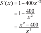
Setting the derivative equal to zero gives you x2 – 400 = 0, and keeping only the positive solution, you have x = 20. You can verify that this value gives you a minimum by using the first derivative test.
Using x = 20 and xy = 400 gives you y = 20.
500. 15 m × 15 m
If you let x and y be the side lengths of the rectangle, you have the following equation for the perimeter:
![]()
The function that you want to maximize, the area, is given by
![]()
You can write this as a function of one variable by using 2x + 2y = 60 to get y = 30 – x. Substituting the value of y into the area equation gives you

Take the derivative and set it equal to zero to find x:
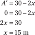
You can verify that this gives you a maximum by using the first derivative test.
Using 2x + 2y = 60 and x = 15 meters, you get y = 15 meters.
501. 56,250 ft2
Let x and y be the lengths of the sides of the pen as in the following diagram:
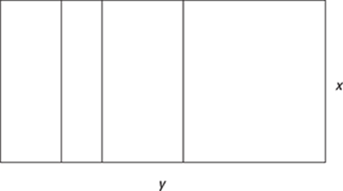
From the diagram, you have the following perimeter formula:
![]()
The function you want to maximize, the area, is given by
![]()
You can write this as a function of one variable by using the equation 5x + 2y = 1,500 to get ![]() . Substituting the value of y into the area equation gives you
. Substituting the value of y into the area equation gives you

Take the derivative of this function, set it equal to zero, and solve for x:
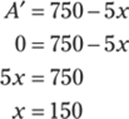
You can verify that this value gives you a maximum by using the first derivative test. Using 5x + 2y = 1,500 and x = 150 gives you y = 375; therefore, the area is
![]()
502. 16 ft3
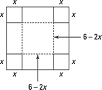
If a square with side x is removed from each corner of the piece of cardboard, you have the following volume, where 0 > x > 3:
![]()
By distributing, you have

You want the maximum volume, so take the derivative of this function:
![]()
Then set the derivative equal to zero and solve for x:
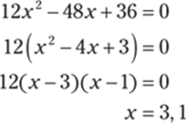
Because x = 3 makes the volume zero, you know that x = 1 gives you a maximum,which you can verify by using the first derivative test.
Using V = (6 – 2x)(6 – 2x)x and x = 1 gives you the volume:

503. ![]() cm ×
cm × ![]() cm ×
cm × ![]() cm
cm
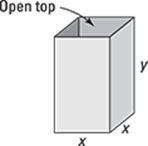
If you let x be a length of one side of the base and let y be the height of the box,the volume is

The square base has an area of x2, and the box has four sides, each with an areaof xy, so the surface area is given by
![]()
You can write this as a function of one variable by using x2y = 16,000 to get ![]() . Substituting the value of y into the surface area formula gives you
. Substituting the value of y into the surface area formula gives you

You want the minimum surface area, so take the derivative of this function:

Then set the derivative equal to zero and solve for x:
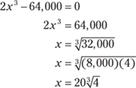
Use ![]() to find y:
to find y:
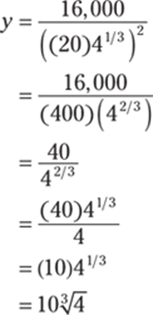
Therefore, the dimensions are ![]() cm ×
cm × ![]() cm ×
cm × ![]() cm (approximately 31.75 cm × 31.75 cm × 15.87 cm).
cm (approximately 31.75 cm × 31.75 cm × 15.87 cm).
Note that you can easily use the second derivative test to verify that ![]() gives you a minimum because S" > 0 for all x > 0.
gives you a minimum because S" > 0 for all x > 0.
504.  ,
, 
You want to find the maximum distance. The distance from a point (x, y) to the point (1, 0) is given by

Rewrite the equation of the ellipse as y2 = 8 – 8x2 and substitute the value of y2 into the distance equation:

Tip: You can take the derivative of this function and use the first derivative test to find a maximum, but it's easier to use the square of the distance, which gets rid of the radical. For a function that satisfies f (x) ≥ 0, its local maxima and minima occur at the same x values as the local maxima and minima of its square, [f (x)]2. Obviously, the corresponding y values would change, but that doesn't matter here!
The square of the distance is
![]()
And the derivative of this function is
![]()
Setting the derivative equal to zero and solving gives you –2 – 14x = 0, or –2 = 14x, which has the solution ![]() . You can verify that
. You can verify that ![]() gives you a maximum by using the first derivative test.
gives you a maximum by using the first derivative test.
Using ![]() and y2 = 8 – 8x2, find the y coordinate:
and y2 = 8 – 8x2, find the y coordinate:
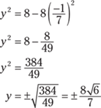
Therefore, the two points that are farthest from (1, 0) are the points  and
and  .
.
505. ![]()
You want to find the minimum distance. The distance from a point (x, y) to the origin is

Using y = 4x + 6, the distance is

Tip: You can take the derivative of this function and use the first derivative test to find a minimum, but it's easier to use the square of the distance, which gets rid of the radical. For a function that satisfies f (x) ≥ 0, its local maxima and minima occur at the same x values as the local maxima and minima of its square, [f (x)]2. Obviously, the corresponding y values would change, but that doesn't matter here!
Using the square of the distance, you have
![]()
The derivative is
![]()
Setting the derivative equal to zero gives you 34x + 48 = 0, which has the solution ![]() . You can verify that this value gives you a minimum by using the first derivative test.
. You can verify that this value gives you a minimum by using the first derivative test.
Using ![]() and y = 4x + 6, find the y coordinate:
and y = 4x + 6, find the y coordinate:
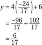
Therefore, the point closest to the origin is ![]() .
.
506. ![]() in. ×
in. × ![]() in.
in.
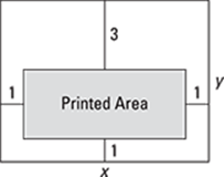
You want to maximize the printed area. Let x and y be the length and width of the poster. Because the total area must be 90 square inches, you have A = xy = 90.
The poster has a 1-inch margin at the bottom and sides and a 3-inch margin at the top, so the printed area of the poster is
![]()
Using ![]() , the printed area is
, the printed area is
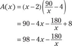
Find the derivative of the function for the printed area:
![]()
Set the derivative equal to zero and solve for x: –4x2 + 180 = 0 so that x2 = 45. Keeping the positive solution, you have ![]() .
.
Using the first derivative test, you can verify that ![]() gives you a maximum. From the equation
gives you a maximum. From the equation ![]() , you get the y value:
, you get the y value:

Therefore, the dimensions are ![]() inches ×
inches × ![]() inches (approximately 6.7 inches ×13.4 inches).
inches (approximately 6.7 inches ×13.4 inches).
507. ![]() and
and ![]()
You want to locate the maximum slope of f (x) = 2 + 20x3 – 4x5. The slope of the tangent line is given by the derivative
![]()
At a point p, the slope is
![]()
You want to maximize this function, so take another derivative:
![]()
To find the critical numbers, set this function equal to zero and solve for p:
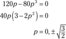
Take a point from each interval and test it in s'(p) to see whether the answer is positive or negative. By taking a point from the interval  , you have s'(p) > 0; by using a point from
  , you have s'(p) > 0; in
  , you have s'(p) > 0; and in
  , you haves'(p) > 0. Because s(p) approaches –∞ as x approaches ±∞, the maximum value must occur at one (or both) of
 ![]() .
.
Substituting these values into the slope equation gives you
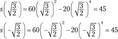
Therefore, the maximum slope occurs when ![]() and when
and when ![]() .
.
508. $396.23
If you let x be the length of the base and let y be the height, the volume is

The area of the base is 2x2, and the box has four sides, each with an area of xy. With the base material at $20 per square meter and the side material at $12 per square meter, the total cost is

You can write this as a function of one variable by using the volume equation to get ![]() . The cost becomes
. The cost becomes

You want the minimum cost, so find the derivative of this function:

Setting this equal to zero, you get 80x3 – 480 = 0, which has the solution ![]() meters. Substituting this value into the cost function C(x) = 40x2 + 480x−1 gives you the minimum cost:
meters. Substituting this value into the cost function C(x) = 40x2 + 480x−1 gives you the minimum cost:

509. 20 m
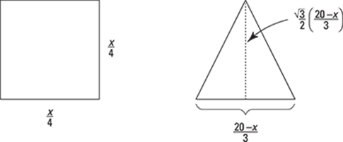
You want to maximize the total area. If x is the length of wire used for the square, each side of the square has a length of ![]() meters, so the area of the square is
meters, so the area of the square is ![]() . You'll have (20 – x) meters of wire left for the triangle, so each side of the triangle is
. You'll have (20 – x) meters of wire left for the triangle, so each side of the triangle is ![]() meters. Because the triangle is equilateral, its height is
meters. Because the triangle is equilateral, its height is  meters, so the area of the triangle is
  . Therefore, the total area of the square and the triangle together is

where 0 ≤ x ≤ 20.
Find the derivative of this function:
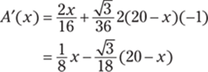
Then set the derivative equal to zero and solve for x:
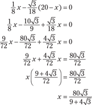
It's reasonable to let x = 0 (the wire is used entirely to make the triangle) or x = 20 (the wire is used entirely to make the square), so check those values as well. Here are the areas:
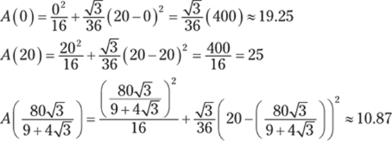
The maximum occurs when x = 20.
510. 

You want to minimize the total area. If x is the length of wire used for the square, each side of the square has a length of ![]() meters, so the area of the square is
meters, so the area of the square is ![]() . You'll have (20 – x) meters of wire left for the triangle, so each side of the triangle is
. You'll have (20 – x) meters of wire left for the triangle, so each side of the triangle is ![]() meters. Because the triangle is equilateral, its height is
meters. Because the triangle is equilateral, its height is  meters, so the area of the triangle is
  . Therefore, the total area of the square and the triangle together is

where 0 ≤ x ≤ 20.
Find the derivative of this function:

Set the derivative equal to zero and solve for x:

It's reasonable to let x = 0 (the wire is used entirely to make the triangle) or x = 20 (the wire is used entirely to make the square), so check those values as well. Here are the areas:

Therefore, the minimum occurs when

511.  feet from the bright light source

Let x be the distance of the object from the brighter light source and k be the strength of the weaker light source. The illumination of each light source is directly proportional to the strength of the light source (5k and k) and inversely proportional to the square of the distance from the source (x and 20 – x), so the total illumination is

where 0 > x > 20.
Taking the derivative of this function gives you
![]()
Set this derivative equal to zero and simplify:

Then solve for x. Taking the cube root of both sides and solving gives you
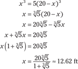
Note that you can use the first derivative test to verify that this value does in fact give a minimum.
512. 12
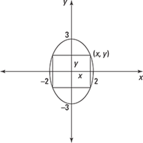
You want to maximize the area of the rectangle. From the diagram, the area of the rectangle is
![]()
Using the equation of the ellipse, solve for x:
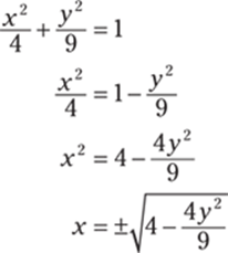
Keeping only the positive solution, you have  (although you can just as easily work with the negative solution). Therefore, the area in terms of y becomes
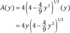
Take the derivative by using the product rule and the chain rule:
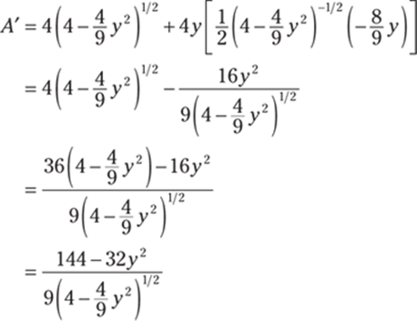
Then set the derivative equal to zero and solve for y:
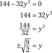
Keeping the positive solution (either works), you have  , which gives you the following x value:
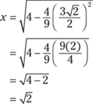
Therefore, the area of the rectangle is

Note that you can verify that the value  does indeed give a maximum by using the first derivative test.
513. 0.84771
Use the formula  with f (x) = x3 + 4x – 4, f '(x) = 3x2 + 4, and x1 = 1. Note that the formula gives you
  ,
,  , and so on. Therefore, you have
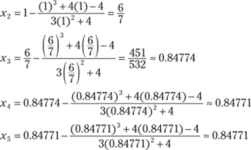
514. 2.0597671
Use the formula  with f (x) = x4 – 18, f '(x) = 4x3, and x1 = 2. Note that the formula gives you
  ,
,  , and so on. Therefore, you have
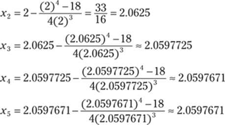
515. –1.2457342
Use the formula  with f (x) = x5 + 3, f '(x) = 5x4, and x1 = –1. Note that the formula gives you
  ,
,  , and so on. Therefore, you have
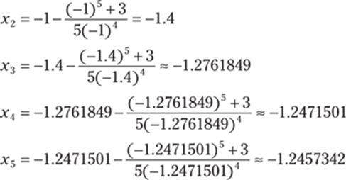
516. 0.73909
Newton's method begins by making one side of the equation zero, labeling the other side f (x), and then picking a value of x1 that's “close” to a root of f (x). There's certainly a bit of trial and error involved; in this case, you could graph both y = cos x and y = x and look for a point of intersection to get a rough idea of what the root may be.
Use the formula  with f (x) = cos x – x and f '(x) = –sin x – 1. Note that the formula gives you
  ,
,  , and so on. You also have to decide on a value for x1. Notice that f (0) = 1 – 0 = 1, which is close to the desired value of 0, so you can start with the value x1 = 0. Therefore, you have
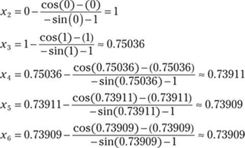
The approximation is no longer changing, so the solution is 0.73909.
517. 1.69562
Newton's method begins by making one side of the equation zero, labeling the other side f (x), and then picking a value of x1 that's “close” to a root of f (x). In general, a bit of trial and error is involved, but in this case, you're given a closed interval to work with, which considerably narrows down the choices!
Use the formula  with f (x) = x3 – x2 – 2 and f '(x) = 3x2– 2x. Note that the formula gives you
  ,
,  , and so on. You can choose any value in the interval [1, 2] for x1, but x1 = 1 makes the computations a bit easier for the first step, so use that value:
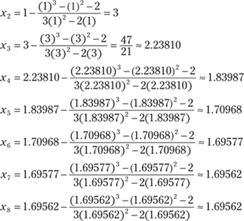
The approximation is no longer changing, so the solution is 1.69562.
518. 1.22074
Newton's method begins by making one side of the equation zero, labeling the other side f (x), and then picking a value of x1 that's “close” to a root of f (x). There's certainly a bit of trial and error involved; in this case, you could graph both ![]() and y = x2 and look for a point of intersection to get a rough idea of what the root may be.
and y = x2 and look for a point of intersection to get a rough idea of what the root may be.
Use the formula  with
with ![]() and
and ![]() . Note that the formula gives you
. Note that the formula gives you  ,
,  , and so on. Notice that
 ![]() , which is close to the desired value of 0, so you can start withx1 = 1:
, which is close to the desired value of 0, so you can start withx1 = 1:
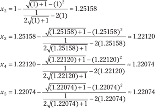
The approximation is no longer changing, so the solution is 1.22074.
519. ![]()
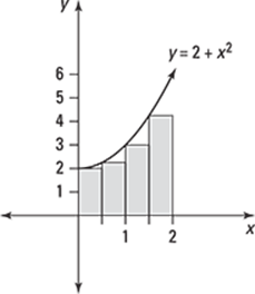
Because the given function has values that are strictly greater than or equal to zero on the given interval, you can interpret the Riemann sum as approximating the area that's underneath the curve and bounded below by the x-axis.
You want to use four rectangles of equal width to estimate the area under f (x) = 2 + x2 over the interval 0 ≤ x ≤ 2. Begin by dividing the length of the interval by 4 to find the width of each rectangle:
![]()
Then divide the interval [0, 2] into 4 equal pieces, each with a width of ![]() , to get the intervals
, to get the intervals ![]() ,
, ![]() ,
, ![]() , and
, and ![]() . Using the left endpoint of each interval to calculate the heights of the rectangles gives you the values x = 0,
. Using the left endpoint of each interval to calculate the heights of the rectangles gives you the values x = 0, ![]() , x = 1, and
, x = 1, and ![]() . The height of each rectangle is f (x). To approximate the area under the curve, multiply the width of each rectangle by f (x) and add the areas:
. The height of each rectangle is f (x). To approximate the area under the curve, multiply the width of each rectangle by f (x) and add the areas:

520. 10.43
Because the given function has values that are strictly greater than or equal to zero on the given interval, you can interpret the Riemann sum as approximating the area that's underneath the curve and bounded below by the x-axis.
You want to use five rectangles of equal width to estimate the area under ![]() over the interval 1 ≤ x ≤ 4. Begin by dividing the length of the interval by 5 to find the width of each rectangle:
over the interval 1 ≤ x ≤ 4. Begin by dividing the length of the interval by 5 to find the width of each rectangle:
![]()
Then divide the interval [1, 4] into 5 equal pieces, each with a width of ![]() , to get the intervals
, to get the intervals ![]() ,
, ![]() ,
, ![]() ,
, ![]() , and
, and ![]() . Using the left endpoint of each interval to calculate the heights of the rectangles gives you the values x = 1,
. Using the left endpoint of each interval to calculate the heights of the rectangles gives you the values x = 1, ![]() ,
, ![]() ,
, ![]() , and
, and ![]() . The height of each rectangle is f (x). To approximate the area under the curve, multiply the width of each rectangle by f (x) and add the areas:
. The height of each rectangle is f (x). To approximate the area under the curve, multiply the width of each rectangle by f (x) and add the areas:

521. 22.66
Because the given function has values that are strictly greater than or equal to zero on the given interval, you can interpret the Riemann sum as approximating the area that's underneath the curve and bounded below by the x-axis.
You want to use seven rectangles of equal width to estimate the area under f (x) = 4 ln x + 2x over the interval 1 ≤ x ≤ 4. Begin by dividing the length of the interval by 7 to find the width of each rectangle:
![]()
Then divide the interval [1, 4] into 7 equal pieces, each with a width of ![]() , to get the intervals
, to get the intervals ![]() ,
, ![]() ,
, ![]() ,
, ![]() ,
, ![]() ,
, ![]() , and
, and ![]() . Using the left endpoint of each interval to calculate the heights of the rectangles gives you the values x = 1,
. Using the left endpoint of each interval to calculate the heights of the rectangles gives you the values x = 1, ![]() ,
, ![]() ,
, ![]() ,
, ![]() ,
, ![]() , and
, and ![]() . The height of each rectangle is f (x). To approximate the area under the curve, multiply the width of each rectangle by f (x) and add the areas:
. The height of each rectangle is f (x). To approximate the area under the curve, multiply the width of each rectangle by f (x) and add the areas:

522. 2.788 × 10¹⁰
Because the given function has values that are strictly greater than or equal to zero on the given interval, you can interpret the Riemann sum as approximating the area that's underneath the curve and bounded below by the x-axis.
You want to use eight rectangles of equal width to estimate the area under f (x) = e3x + 4 over the interval 1 ≤ x ≤ 9. Begin by dividing the length of the interval by 8 to find the width of each rectangle:
![]()
Then divide the interval [1, 9] into 8 equal pieces, each with a width of 1, to get the intervals [1, 2], [2, 3], [3, 4], [4, 5], [5, 6], [6, 7], [7, 8], and [8, 9]. Using the left endpoint of each interval to calculate the heights of the rectangles gives you the values x = 1, x = 2, x = 3, x = 4, x = 5,x = 6, x = 7, and x = 8. The height of each rectangle is f (x). To approximate the area under the curve, multiply the width of each rectangle by f (x) and add the areas:

523. 24
Because the given function has values that are strictly greater than or equal to zero on the given interval, you can interpret the Riemann sum as approximating the area that's underneath the curve and bounded below by the x-axis.
You want to use four rectangles of equal width to estimate the area under f (x) = 1 + 2x over the interval 0 ≤ x ≤ 4. Begin by dividing the length of the interval by 4 to find the width of each rectangle:
![]()
Then divide the interval [0, 4] into 4 equal pieces, each with a width of 1, to get the intervals [0, 1], [1, 2], [2, 3], and [3, 4]. Using the right endpoint of each interval to calculate the heights of the rectangles gives you the values x = 1, x = 2, x = 3, and x = 4.The height of each rectangle is f (x). To approximate the area under the curve, multiply the width of each rectangle by f (x) and add the areas:

524. –8.89
In this example, the given function has values that are both positive and negative on the given interval, so don't make the mistake of thinking the Riemann sum approximates the area between the curve and the x-axis. In this case, the Riemann sum approximates the value of

You want to use five rectangles of equal width over the interval 2 ≤ x ≤ 6. Begin by dividing the length of the interval by 5 to find the width of each rectangle:
![]()
Then divide the interval [2, 6] into 5 equal pieces, each with a width of ![]() , to get the intervals
, to get the intervals ![]() ,
, ![]() ,
, ![]() ,
, ![]() , and
, and ![]() . Using the right endpoint of each interval to calculate the heights of the rectangles gives you the values
. Using the right endpoint of each interval to calculate the heights of the rectangles gives you the values ![]() ,
, ![]() ,
, ![]() ,
, ![]() , and x = 6. The height of each rectangle is f (x). (Note that a “negative height” indicates that the rectangle is below the x-axis.) To find the Riemann sum, multiply the width of each rectangle by f (x) and add the areas:
, and x = 6. The height of each rectangle is f (x). (Note that a “negative height” indicates that the rectangle is below the x-axis.) To find the Riemann sum, multiply the width of each rectangle by f (x) and add the areas:

525. 3.24
In this example, the given function has values that are both positive and negative on the given interval, so the Riemann sum approximates the value of

You want to use six rectangles of equal width over the interval 0 ≤ x ≤ 5. Begin by dividing the length of the interval by 6 to find the width of each rectangle:
![]()
Then divide the interval [0, 5] into 6 equal pieces, each with a width of ![]() , to get the intervals
, to get the intervals ![]() ,
, ![]() ,
, ![]() ,
, ![]() ,
, ![]() , and
, and ![]() . Using the right endpoint of each interval to calculate the height of the rectangles gives you the values
. Using the right endpoint of each interval to calculate the height of the rectangles gives you the values ![]() ,
, ![]() ,
, ![]() ,
, ![]() ,
, ![]() , and x = 5. The height of each rectangle is f (x). (Note that a “negative height” indicates that the rectangle is below the x-axis.) To find the Riemann sum, multiply the width of each rectangle by f (x) and add the areas:
, and x = 5. The height of each rectangle is f (x). (Note that a “negative height” indicates that the rectangle is below the x-axis.) To find the Riemann sum, multiply the width of each rectangle by f (x) and add the areas:

526. 1.34
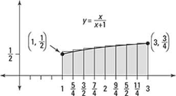
Because the given function has values that are strictly greater than or equal to zero on the given interval, you can interpret the Riemann sum as approximating the area that's underneath the curve and bounded below by the x-axis.
You want to use eight rectangles of equal width to estimate the area under ![]() over the interval 1 ≤ x ≤ 3. Begin by dividing the length of the interval by 8 to find the width of each rectangle:
over the interval 1 ≤ x ≤ 3. Begin by dividing the length of the interval by 8 to find the width of each rectangle:
![]()
Then divide the interval [1, 3] into eight equal pieces, each with a width of ![]() , to get the intervals
, to get the intervals ![]() ,
, ![]() ,
, ![]() ,
, ![]() ,
, ![]() ,
, ![]() ,
, ![]() , and
, and ![]() . Using the right endpoint of each interval to calculate the height of the rectangles gives you the values
. Using the right endpoint of each interval to calculate the height of the rectangles gives you the values ![]() ,
, ![]() ,
, ![]() , x = 2,
, x = 2, ![]() ,
, ![]() ,
, ![]() , and x = 3. The height of each rectangle is f (x). To approximate the area under the curve, multiply the width of each rectangle by f (x) and add the areas:
, and x = 3. The height of each rectangle is f (x). To approximate the area under the curve, multiply the width of each rectangle by f (x) and add the areas:
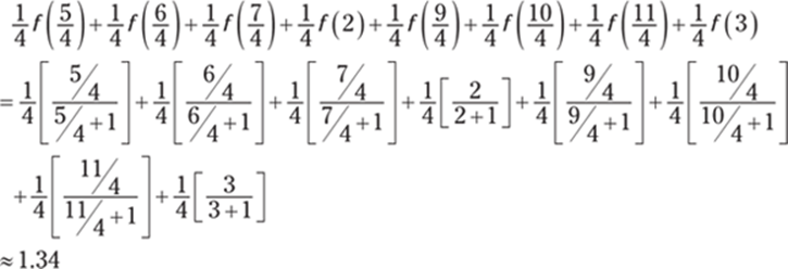
527. 0.29
In this example, the given function has values that are both positive and negative on the given interval, so don't make the mistake of thinking the Riemann sum approximates the area between the curve and the x-axis. In this case, the Riemann sum approximates the value of

You want to use four rectangles of equal width over the interval 0 ≤ x ≤ 3. Begin by dividing the length of the interval by 4 to find the width of each rectangle:
![]()
Then divide the interval [0, 3] into 4 equal pieces, each with a width of ![]() , to get the intervals
, to get the intervals ![]() ,
, ![]() ,
, ![]() , and
, and ![]() . Recall that to find the midpoint of an interval, you simply add the left and the right endpoints together and then divide by 2 (that is, you average the two values). In this case, the midpoints are
. Recall that to find the midpoint of an interval, you simply add the left and the right endpoints together and then divide by 2 (that is, you average the two values). In this case, the midpoints are ![]() ,
, ![]() ,
, ![]() , and
, and ![]() . The height of each rectangle is f (x). (Note that a “negative height” indicates that the rectangle is below the x-axis.) To find the Riemann sum, multiply the width of each rectangle by f (x) and add the areas:
. The height of each rectangle is f (x). (Note that a “negative height” indicates that the rectangle is below the x-axis.) To find the Riemann sum, multiply the width of each rectangle by f (x) and add the areas:

528. 0.32
In this example, the given function has values that are both positive and negative on the given interval, so the Riemann sum approximates the value of

You want to use five rectangles of equal width over the interval 1 ≤ x ≤ 5. Begin by dividing the length of the interval by 5 to find the width of each rectangle:
![]()
Divide the interval [1, 5] into 5 equal pieces, each with a width of ![]() , to get the intervals
, to get the intervals ![]() ,
, ![]() ,
, ![]() ,
, ![]() , and
, and ![]() . Recall that to find the midpoint of an interval, you simply add the left and the right endpoints together and then divide by 2 (that is, you average the two values). In this case, the midpoints are
. Recall that to find the midpoint of an interval, you simply add the left and the right endpoints together and then divide by 2 (that is, you average the two values). In this case, the midpoints are ![]() ,
, ![]() ,
, ![]() ,
, ![]() , and
, and ![]() . The height of each rectangle is f (x). (Note that a “negative height” indicates that the rectangle is below the x-axis.) To find the Riemann sum, multiply the width of each rectangle by f (x) and add the areas:
. The height of each rectangle is f (x). (Note that a “negative height” indicates that the rectangle is below the x-axis.) To find the Riemann sum, multiply the width of each rectangle by f (x) and add the areas:

529. 160.03
Because the given function has values that are strictly greater than or equal to zero on the given interval, you can interpret the Riemann sum as approximating the area that's underneath the curve and bounded below by the x-axis.
You want to use six rectangles of equal width over the interval 1 ≤ x ≤ 3. Begin by dividing the length of the interval by 6 to find the width of each rectangle:
![]()
Then divide the interval [1, 4] into 6 equal pieces, each with a width of ![]() , to get the intervals
, to get the intervals ![]() ,
, ![]() ,
, ![]() ,
, ![]() ,
, ![]() , and
, and ![]() . Recall that to find the midpoint of an interval, you simply add the left and the right endpoints together and then divide by 2 (that is, you average the two values). In this case, the midpoints are
. Recall that to find the midpoint of an interval, you simply add the left and the right endpoints together and then divide by 2 (that is, you average the two values). In this case, the midpoints are ![]() ,
, ![]() ,
, ![]() ,
, ![]() ,
, ![]() , and
, and ![]() . The height of each rectangle is f (x). To find the Riemann sum, multiply the width of each rectangle by f (x) and add the areas:
. The height of each rectangle is f (x). To find the Riemann sum, multiply the width of each rectangle by f (x) and add the areas:

530. 18.79
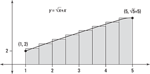
Because the given function has values that are strictly greater than or equal to zero on the given interval, you can interpret the Riemann sum as approximating the area that's underneath the curve and bounded below by the x-axis.
You want to use eight rectangles of equal width over the interval 1 ≤ x ≤ 5. Begin by dividing the length of the interval by 8 to find the width of each rectangle:
![]()
Then divide the interval [1, 5] into 8 equal pieces, each with a width of ![]() , to get the intervals
, to get the intervals ![]() ,
, ![]() ,
, ![]() ,
, ![]() ,
, ![]() ,
, ![]() ,
, ![]() , and
, and ![]() . Recall that to find the midpoint of an interval, you simply add the left and the right endpoints together and then divide by 2 (that is, you average the two values). In this case, the midpoints are
. Recall that to find the midpoint of an interval, you simply add the left and the right endpoints together and then divide by 2 (that is, you average the two values). In this case, the midpoints are ![]() ,
, ![]() ,
, ![]() ,
, ![]() ,
, ![]() ,
, ![]() ,
, ![]() , and
, and ![]() . The height of each rectangle is f (x). To approximate the area under the curve, multiply the width of each rectangle by f (x) and add the areas:
. The height of each rectangle is f (x). To approximate the area under the curve, multiply the width of each rectangle by f (x) and add the areas:

531. 
To begin, you split the interval into n pieces of equal width using the formula ![]() , where a is the lower limit of integration and b is the upper limit of integration. In this case, you have
, where a is the lower limit of integration and b is the upper limit of integration. In this case, you have
![]()
You also want to select a point from each interval. The formula xi = a + (Δx)i gives you the right endpoint from each interval. Here, you have
![]()
Substituting those values into the definition of the definite integral gives you
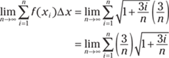
532. ![]()
To begin, you split the interval into n pieces of equal width using the formula ![]() , where a is the lower limit of integration and b is the upper limit of integration. In this case, you have
, where a is the lower limit of integration and b is the upper limit of integration. In this case, you have
![]()
You also want to select a point from each interval. The formula xi = a + (Δx)i gives you the right endpoint from each interval. Here, you have
![]()
Substituting those values into the definition of the definite integral gives you

533. 
To begin, you split the interval into n pieces of equal width using the formula ![]() , where a is the lower limit of integration and b is the upper limit of integration. In this case, you have
, where a is the lower limit of integration and b is the upper limit of integration. In this case, you have
![]()
You also want to select a point from each interval. The formula xi = a + (Δx)i gives you the right endpoint from each interval. Here, you have
![]()
Substituting those values into the definition of the definite integral gives you

534. 
To begin, you split the interval into n pieces of equal width using the formula ![]() , where a is the lower limit of integration and b is the upper limit of integration. In this case, you have
, where a is the lower limit of integration and b is the upper limit of integration. In this case, you have

You also want to select a point from each interval. The formula xi = a + (Δx)i gives you the right endpoint from each interval. Here, you have
![]()
Substituting those values into the definition of the definite integral gives you

535. 
To begin, you split the interval into n pieces of equal width using the formula ![]() , where a is the lower limit of integration and b is the upper limit of integration. In this case, you have
, where a is the lower limit of integration and b is the upper limit of integration. In this case, you have
![]()
You also want to select a point from each interval. The formula xi = a + (Δx)i gives you the right endpoint from each interval. Here, you have
![]()
Substituting those values into the definition of the definite integral gives you
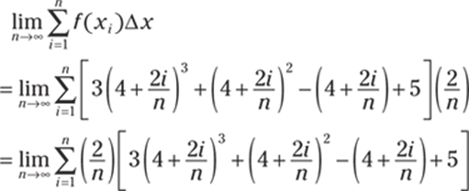
536. ![]()
Recall that in the limit representation of a definite integral, you divide the interval over which you're integrating into n pieces of equal width. You also have to select a point from each interval; the formula a + (Δx)i lets you select the right endpoint of each interval.
Begin by looking for the factor that would represent Δx. In this example, ![]() ; if you ignore the n in this expression, you're left with the length of the interval over which the definite integral is being evaluated. In this case, the length of the interval is 3. Notice that if you consider
; if you ignore the n in this expression, you're left with the length of the interval over which the definite integral is being evaluated. In this case, the length of the interval is 3. Notice that if you consider ![]() , this is of the form a + (Δx)i, where a = 4.
, this is of the form a + (Δx)i, where a = 4.
You now have a value for a and know the length of the interval, so you can conclude that you're integrating over the interval [4, 7]. To produce the function, replace each expression of the form ![]() that appears in the summation with the variable x. In this example, you replace
that appears in the summation with the variable x. In this example, you replace  with x6 so that f (x) = x6. Therefore, the Riemann sum could represent the definite integral
 ![]() .
.
537. ![]()
Recall that in the limit representation of a definite integral, you divide the interval over which you're integrating into n pieces of equal width. You also have to select a point from each interval; the formula a + (Δx)i lets you select the right endpoint of each interval.
Begin by looking for the factor that would represent Δx. In this example, ![]() ; if you ignore the n in this expression, you're left with the length of the interval over which the definite integral is being evaluated. In this case, the length of the interval is
; if you ignore the n in this expression, you're left with the length of the interval over which the definite integral is being evaluated. In this case, the length of the interval is ![]() . Notice that if you consider
. Notice that if you consider ![]() , this is of the form a + (Δx)i, where a = 0.
, this is of the form a + (Δx)i, where a = 0.
You now have a value for a and know the length of the interval, so you can conclude that you're integrating over the interval ![]() . To produce the function, replace each expression of the form
. To produce the function, replace each expression of the form ![]() that appears in the summation with the variable x. In this example, you replace
that appears in the summation with the variable x. In this example, you replace ![]() with sec x so that f (x) = sec x. Therefore, the Riemann sum could represent the definite integral
with sec x so that f (x) = sec x. Therefore, the Riemann sum could represent the definite integral ![]() .
.
538. ![]()
Recall that in the limit representation of a definite integral, you divide the interval over which you're integrating into n pieces of equal width. You also have to select a point from each interval; the formula a + (Δx)i lets you select the right endpoint of each interval.
Begin by looking for the factor that would represent Δx. In this example, ![]() ; if you ignore the n in this expression, you're left with the length of the interval over which the definite integral is being evaluated. In this case, the length of the interval is 1. Notice that if you consider
; if you ignore the n in this expression, you're left with the length of the interval over which the definite integral is being evaluated. In this case, the length of the interval is 1. Notice that if you consider ![]() , this is of the form a + (Δx)i, where a = 6.
, this is of the form a + (Δx)i, where a = 6.
You now have a value for a and know the length of the interval, so you can conclude that you're integrating over the interval [6, 7]. To produce the function, replace each expression of the form ![]() that appears in the summation with the variable x. In this example, you replace
that appears in the summation with the variable x. In this example, you replace ![]() with x so that f (x) = x. Therefore, the Riemann sum could represent the definite integral
with x so that f (x) = x. Therefore, the Riemann sum could represent the definite integral ![]() .
.
539. ![]()
Recall that in the limit representation of a definite integral, you divide the interval over which you're integrating into n pieces of equal width. You also have to select a point from each interval; the formula a + (Δx)i lets you select the right endpoint of each interval.
Begin by looking for the factor that would represent Δx. In this example, ![]() ; if you ignore the n in this expression, you're left with the length of the interval over which the definite integral is being evaluated. In this case, the length of the interval is
; if you ignore the n in this expression, you're left with the length of the interval over which the definite integral is being evaluated. In this case, the length of the interval is ![]() . Notice that if you consider
. Notice that if you consider ![]() , this is of the form a + (Δx)i, where a = 0.
, this is of the form a + (Δx)i, where a = 0.
You now have a value for a and know the length of the interval, so you can conclude that you're integrating over the interval ![]() . To produce the function, replace each expression of the form
. To produce the function, replace each expression of the form ![]() that appears in the summation with the variable x. In this example, you replace
that appears in the summation with the variable x. In this example, you replace ![]() with cos x + sin x so that f (x) = cos x + sin x. Therefore, the Riemann sum could represent the definite integral
with cos x + sin x so that f (x) = cos x + sin x. Therefore, the Riemann sum could represent the definite integral ![]() .
.
540. ![]()
Recall that in the limit representation of a definite integral, you divide the interval over which you're integrating into n pieces of equal width. You also have to select a point from each interval; the formula a + (Δx)i lets you select the right endpoint of each interval.
Begin by looking for the factor that would represent Δx. In this example, ![]() ; if you ignore the n in this expression, you're left with the length of the interval over which the definite integral is being evaluated. In this case, the length of the interval is 5. Notice that if you consider
; if you ignore the n in this expression, you're left with the length of the interval over which the definite integral is being evaluated. In this case, the length of the interval is 5. Notice that if you consider ![]() , this is of the form a + (Δx)i, where a = 0.
, this is of the form a + (Δx)i, where a = 0.
You now have a value for a and know the length of the interval, so you can conclude that you're integrating over the interval [0, 5]. To produce the function, replace each expression of the form ![]() that appears in the summation with the variable x. Notice that you can rewrite the summation as
that appears in the summation with the variable x. Notice that you can rewrite the summation as  ; that means you can replace
  with
with ![]() so that
so that ![]() . Therefore, the Riemann sum could represent the definite integral
. Therefore, the Riemann sum could represent the definite integral ![]() .
.
541. 6
To begin, you split the interval into n pieces of equal width using the formula ![]() , where a is the lower limit of integration and b is the upper limit of integration. In this case, you have
, where a is the lower limit of integration and b is the upper limit of integration. In this case, you have
![]()
You also want to select a point from each interval. The formula xi = a + (Δx)i gives you the right endpoint from each interval. Here, you have
![]()
Substituting those values into the definition of the integral gives you the following:
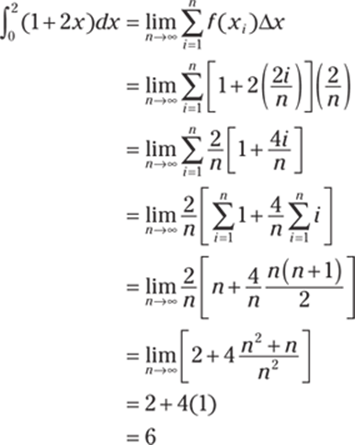
Note that formulas ![]() and
and  were used to simplify the summations.
542. 196
To begin, you split the interval into n pieces of equal width using the formula ![]() , where a is the lower limit of integration and b is the upper limit of integration. In this case, you have
, where a is the lower limit of integration and b is the upper limit of integration. In this case, you have
![]()
You also want to select a point from each interval. The formula xi = a + (Δx)i gives you the right endpoint from each interval. Here, you have
![]()
Substituting those values into the definition of the integral gives you the following:
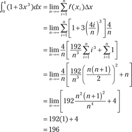
Note that the formulas ![]() and
and  were used to simplify the summations.
543. ![]()
To begin, you split the interval into n pieces of equal width using the formula ![]() , where a is the lower limit of integration and b is the upper limit of integration. In this case, you have
, where a is the lower limit of integration and b is the upper limit of integration. In this case, you have
![]()
You also want to select a point from each interval. The formula xi = a + (Δx)i gives you the right endpoint from each interval. Here, you have
![]()
Substituting those values into the definition of the integral gives you the following:
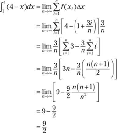
Note that the formulas ![]() and
and  were used to simplify the summations.
544. ![]()
To begin, you split the interval into n pieces of equal width using the formula ![]() , where a is the lower limit of integration and b is the upper limit of integration. In this case, you have
, where a is the lower limit of integration and b is the upper limit of integration. In this case, you have
![]()
You also want to select a point from each interval. The formula xi = a + (Δx)i gives you the right endpoint from each interval. Here, you have
![]()
Substituting those values into the definition of the integral gives you the following:
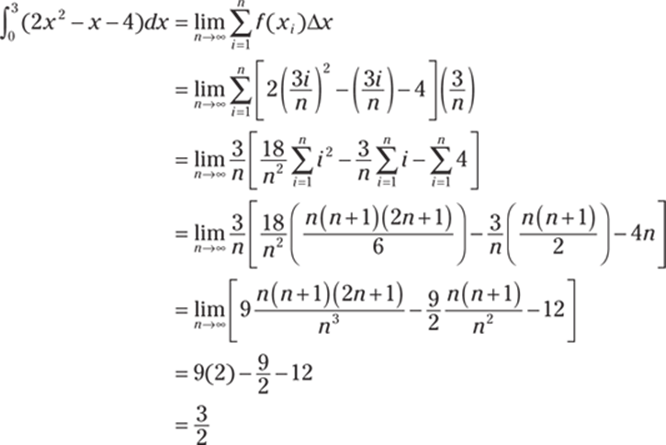
Note that the formulas ![]() ,
,  , and
, and  were used to simplify the summations.
545. ![]()
To begin, you split the interval into n pieces of equal width using the formula ![]() , where a is the lower limit of integration and b is the upper limit of integration. In this case, you have
, where a is the lower limit of integration and b is the upper limit of integration. In this case, you have
![]()
You also want to select a point from each interval. The formula xi = a + (Δx)i gives you the right endpoint from each interval. Here, you have
![]()
Substituting those values into the definition of the integral gives you the following:
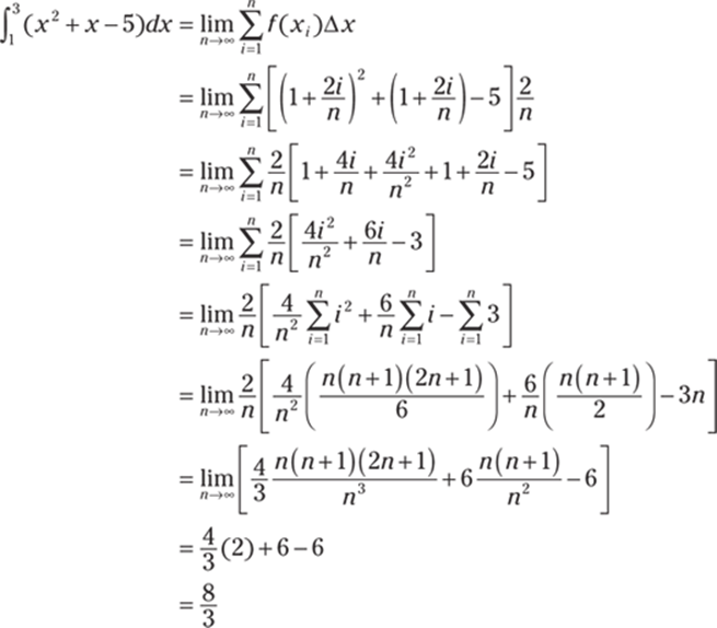
Note that the formulas  ,
,  , and
, and  were used to simplify the summations.
546. ![]()
Part of the fundamental theorem of calculus states that if the function g is continuous on [a, b], then the function f defined by
![]()
is continuous on [a, b] and is differentiable on (a, b). Furthermore, f'(x) = g(x).
To find the derivative of the function ![]() , simply substitute the upper limit of integration, x, into the integrand:
, simply substitute the upper limit of integration, x, into the integrand:
![]()
547. ![]()
To find the derivative of the function ![]() , simply substitute the upper limit of integration, x, into the integrand:
, simply substitute the upper limit of integration, x, into the integrand:
![]()
548. x3 cos x
To find the derivative of the function ![]() , simply substitute the upper limit of integration, x, into the integrand:
, simply substitute the upper limit of integration, x, into the integrand:
![]()
549. ![]()
Part of the fundamental theorem of calculus states that if the function g is continuous on [a, b], then the function f defined by
![]()
is continuous on [a, b] and is differentiable on (a, b). Furthermore, f'(x) = g(x).
To use the fundamental theorem of calculus, you need to have the variable in the upper limit of integration. Therefore, to find the derivative of the function ![]() , first flip the limits of integration and change the sign:
, first flip the limits of integration and change the sign:

Then substitute the upper limit of integration into the integrand to find the derivative:

550. –cos3 x
Part of the fundamental theorem of calculus states that if the function g is continuous on [a, b], then the function f defined by
![]()
is continuous on [a, b] and is differentiable on (a, b). Furthermore, f'(x) = g(x).
To use the fundamental theorem of calculus, you need to have the variable in the upper limit of integration. Therefore, to find the derivative of the function ![]() , first flip the limits of integration and change the sign:
, first flip the limits of integration and change the sign:

Note also that to find ![]() , you can use the substitution u = h(x) and then apply the chain rule as follows:
, you can use the substitution u = h(x) and then apply the chain rule as follows:
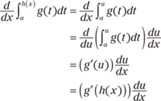
All this tells you to substitute the upper limit of integration into the integrand and multiply by the derivative of the upper limit of integration. Therefore, the derivative of ![]() is
is
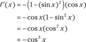
Note that the identity 1 – sin2 x = cos2 x was used to simplify the derivative.
551. –2x
Part of the fundamental theorem of calculus states that if the function g is continuous on [a, b], then the function f defined by
![]()
is continuous on [a, b] and is differentiable on (a, b). Furthermore, f'(x) = g(x).
To use the fundamental theorem of calculus, you need to have the variable in the upper limit of integration. Therefore, to find the derivative of the function ![]() , flip the limits of integration and change the sign of the integral:
, flip the limits of integration and change the sign of the integral:

Note also that to find ![]() , you can use the substitution u = h(x) and then apply the chain rule as follows:
, you can use the substitution u = h(x) and then apply the chain rule as follows:
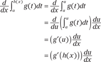
All this tells you to substitute the upper limit of integration into the integrand and multiply by the derivative of the upper limit of integration. Therefore, the derivative of ![]() is
is
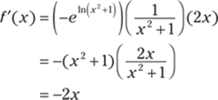
552. ![]()
Part of the fundamental theorem of calculus states that if the function g is continuous on [a, b], then the function f defined by
![]()
is continuous on [a, b] and is differentiable on (a, b). Furthermore, f'(x) = g(x).
To use the fundamental theorem of calculus, you need to have the variable in the upper limit of integration. Therefore, to find the derivative of the function ![]() , first flip the limits of integration and change the sign:
, first flip the limits of integration and change the sign:

Note also that to find ![]() , you can use the substitution
, you can use the substitution
u = h(x) and then apply the chain rule as follows:

All this tells you to substitute the upper limit of integration into the integrand and multiply by the derivative of the upper limit of integration. Therefore, the derivative of ![]() is
is

553. 
Part of the fundamental theorem of calculus states that if the function g is continuous on [a, b], then the function f defined by
![]()
is continuous on [a, b] and is differentiable on (a, b). Furthermore, f'(x) = g(x).
To use the fundamental theorem of calculus, you need to have the variable in the upper limit of integration. Therefore, to find the derivative of the function ![]() , first flip the limits of integration and change the sign:
, first flip the limits of integration and change the sign:

Note also that to find ![]() , you can use the substitution u = h(x) and then apply the chain rule as follows:
, you can use the substitution u = h(x) and then apply the chain rule as follows:

All this tells you to substitute the upper limit of integration into the integrand and multiply by the derivative of the upper limit of integration. Therefore, the derivative of ![]() is
is
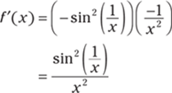
554. ![]()
Part of the fundamental theorem of calculus states that if the function g is continuous on [a, b], then the function f defined by
![]()
is continuous on [a, b] and is differentiable on (a, b). Furthermore, f'(x) = g(x).
Note also that to find ![]() , you can use the substitution u = h(x) and then apply the chain rule as follows:
, you can use the substitution u = h(x) and then apply the chain rule as follows:

All this tells you to substitute the upper limit of integration into the integrand and multiply by the derivative of the upper limit of integration. Therefore, the derivative of ![]() is
is
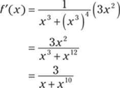
555. 
Part of the fundamental theorem of calculus states that if the function g is continuous on [a, b], then the function f defined by
![]()
is continuous on [a, b] and is differentiable on (a, b). Furthermore, f'(x) = g(x).
To use the fundamental theorem of calculus, you need to have the variable in the upper limit of integration. Therefore, to find the derivative of the function  , first split the integral into two separate integrals:

Then flip the limits of integration and change the sign of the first integral:

Note also that to find ![]() , you can use the substitution u = h(x) and then apply the chain rule as follows:
, you can use the substitution u = h(x) and then apply the chain rule as follows:

All this tells you to substitute the upper limit of integration into the integrand and multiply by the derivative of the upper limit of integration. Therefore, the derivative of  is
is

556. 
Part of the fundamental theorem of calculus states that if the function g is continuous on [a, b], then the function f defined by
![]()
is continuous on [a, b] and is differentiable on (a, b). Furthermore, f'(x) = g(x).
To use the fundamental theorem of calculus, you need to have the variable in the upper limit of integration. Therefore, to find the derivative of the function ![]() , first split the integral into two separate integrals:
, first split the integral into two separate integrals:
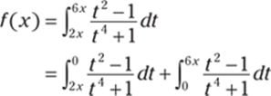
Then flip the limits of integration and change the sign of the first integral:
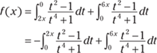
Note also that to find ![]() , you can use the substitution u = h(x) and then apply the chain rule as follows:
, you can use the substitution u = h(x) and then apply the chain rule as follows:

All this tells you to substitute the upper limit of integration into the integrand and multiply by the derivative of the upper limit of integration. Therefore, the derivative of ![]() is
is

557. ![]()
Part of the fundamental theorem of calculus states that if the function g is continuous on [a, b], then the function f defined by
![]()
is continuous on [a, b] and is differentiable on (a, b). Furthermore, f'(x) = g(x).
To use the fundamental theorem of calculus, you need to have the variable in the upper limit of integration. Therefore, to find the derivative of the function ![]() , first split the integral into two separate integrals:
, first split the integral into two separate integrals:

Then flip the limits of integration and change the sign of the first integral:

Note also that to find ![]() , you can use the substitution u = h(x) and then apply the chain rule as follows:
, you can use the substitution u = h(x) and then apply the chain rule as follows:
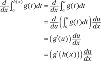
All this tells you to substitute the upper limit of integration into the integrand and multiply by the derivative of the upper limit of integration. Therefore, the derivative of ![]() is
is
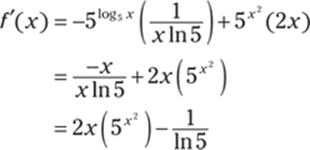
558. 10
Using elementary antiderivative formulas gives you
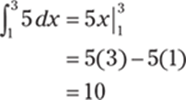
559. ![]()
Using elementary antiderivative formulas gives you
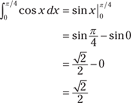
560. 1
Using elementary antiderivative formulas gives you
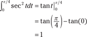
561. 1
Using elementary antiderivative formulas gives you
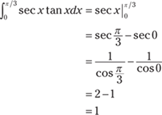
562. ![]()
Using the basic antiderivative formula for an exponential function gives you
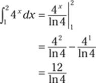
563. ![]()
Using elementary antiderivative formulas gives you
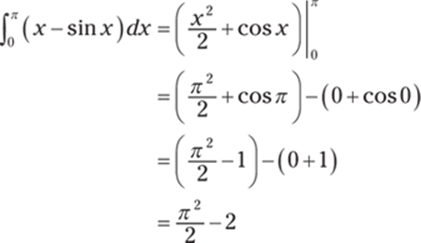
564. ![]()
Using elementary antiderivative formulas gives you
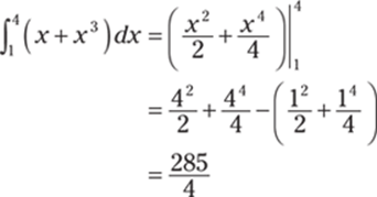
565. ![]()
Rewrite the radical using exponential notation:
![]()
Then use elementary antiderivative formulas:
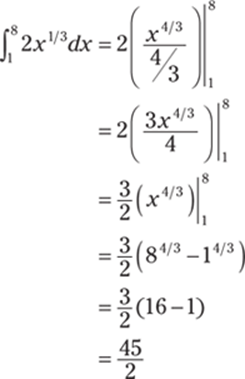
566. ![]()
Using elementary antiderivative formulas gives you
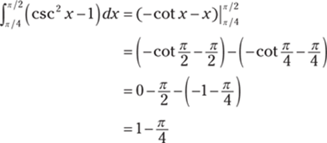
567. –10
Using elementary antiderivative formulas gives you
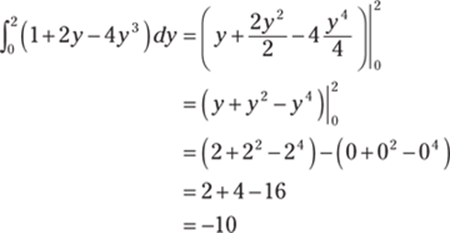
568. ![]()
Begin by rewriting the square root using an exponent:
![]()
Then use elementary antiderivative formulas:
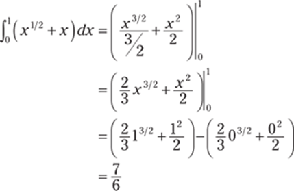
569. ![]()
Integrate each piece of the function over the given integral. Here's the piecewise function:

And here are the calculations:
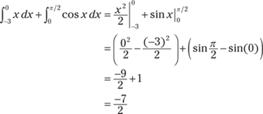
570. ![]()
The given integral is
![]()
Begin by splitting up the integral by using the definition of the absolute value function:

So to evaluate ![]() , use the function –(x – 2) over the interval [–3, 2] and use the function (x – 2) over the interval [2, 4].
, use the function –(x – 2) over the interval [–3, 2] and use the function (x – 2) over the interval [2, 4].
Therefore, the integral becomes
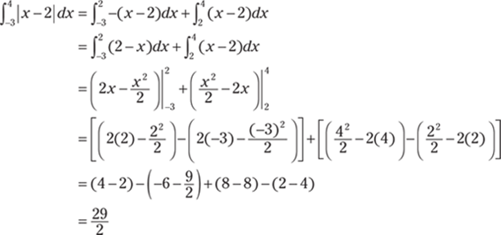
571. ![]()
Add 1 to the exponent and divide by that new exponent to get the antiderivative:
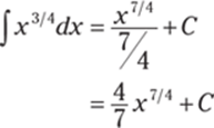
572. ![]()
First move the variable to the numerator:

Then integrate by adding 1 to the exponent while dividing by that new exponent:
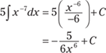
573. ![]()
Find the antiderivative of each term:

574. 3 sin x + 4 cos x + C
Use elementary antiderivative formulas:
![]()
575. 4x + C
This problem can be a bit difficult, unless you remember the trigonometric identities! In this problem, simply factor out the 4 and use a trigonometric identity:

576. tan x – x + C
Use a trigonometric identity followed by elementary antiderivatives:

577. x3 + x2 + x + C
Find the antiderivative of each term:

578. ![]()
Use elementary antiderivative formulas:

579. ![]()
Begin by using a trigonometric identity to replace tan2 x. Then simplify:

580. ![]()
Begin by rewriting the radicals using exponential notation. Then use an elementary antiderivative formula and simplify:
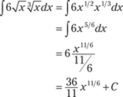
581. ![]()
Rewrite the integrand using exponential notation and factor out the constant. Then use elementary antiderivative formulas:
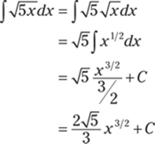
582. ![]()
Begin by writing the radical using exponential notation:
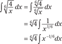
Then use an elementary antiderivative formula:
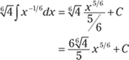
583. ![]()
Use a trigonometric identity in the numerator of the integrand and simplify:
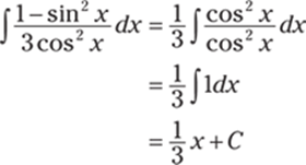
584. ![]()
Begin by multiplying out the integrand. Then integrate each term:
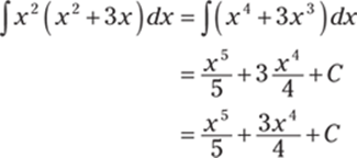
585. ![]()
Begin by breaking up the fraction and simplifying each term:

Then find the antiderivative of each term:

586. ![]()
Expand the integrand and use elementary antiderivative formulas:
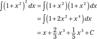
587. 3x + cot x + C
Use a trigonometric identity on the integrand and simplify:

588. ![]()
Begin by splitting up the fraction and writing the radical using exponential notation:

Then use elementary antiderivative formulas and simplify:

589. ![]()
Begin by writing the cube root using exponential notation and multiplying out the integrand:

Then use elementary antiderivative formulas:

590. ![]()
Begin by rewriting the radicals using exponential notation and then distribute:
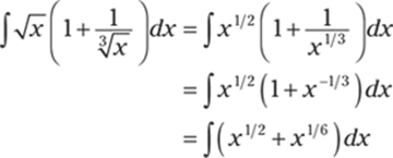
Next, use elementary antiderivative formulas for each term:

591. –csc x + C
Rewrite the integrand. Then use trigonometric identities followed by using a basic antiderivative formula:
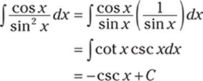
592. ![]()
Begin by splitting up the fraction and simplifying the integrand:

Then use elementary antiderivative formulas:

593. ![]()
Begin by splitting up the fraction and simplifying the integrand:

Then use elementary antiderivative formulas:

594. –cot x + x + C
Begin by splitting up the fraction and using trigonometric identities to rewrite the integrand:

Now apply elementary antiderivative formulas:

595. ![]()
Multiply out the integrand and then use elementary antiderivative formulas on each term:

596. tan x – x + C
Begin by multiplying out the integrand. Then simplify and use elementary antiderivative formulas:

597. ![]()
Factor the numerator out of the integrand. Then simplify and use elementary antiderivative formulas:
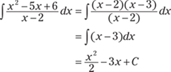
598. ![]()
Begin by factoring the numerator. Then simplify and use elementary antiderivative formulas:
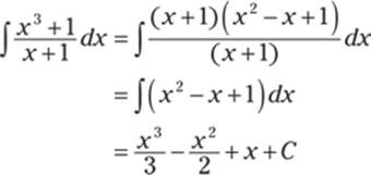
599. ![]()
When finding the antiderivative, don't be thrown off by the decimal exponents; simply add 1 to the exponent of each term and divide by that new exponent for each term to get the solution:
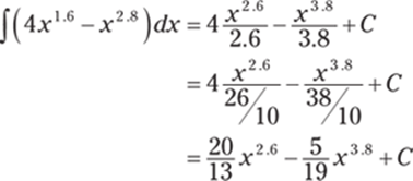
600. ![]()
Begin by splitting up the fraction and simplifying:

Then use elementary antiderivative formulas. To get the final answer, turn the decimals in the denominators into fractions and simplify:

601. ![]()
Start by bringing all variables to the numerator. Then use elementary antiderivative formulas:
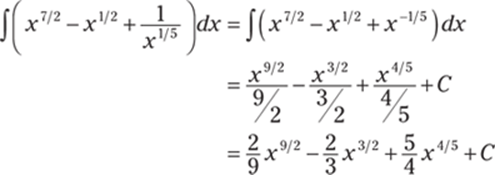
602. ![]()
Use a trigonometric identity and simplify:
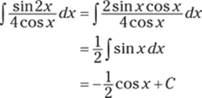
603. x + C
Start by using a trigonometric identity for 1 + cot2 x, followed by rewriting csc2 x as ![]() . Then simplify:
. Then simplify:
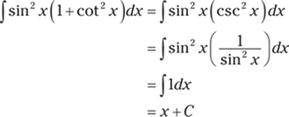
604. ![]()
Begin by splitting the fraction into three terms:

Then use elementary antiderivative formulas and simplify:

605. 7x + C
Begin by factoring the 3 out of the first two terms of the integrand. Then use a trigonometric identity:
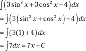
606. ![]()
Begin by factoring the numerator. Then simplify and use elementary antiderivative formulas:
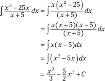
607. tan x + C
Begin by writing tan2 x as ![]() . Then simplify:
. Then simplify:
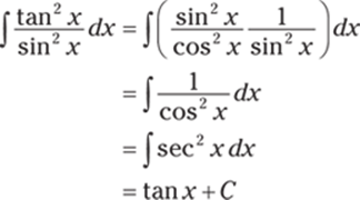
608. sin x + cos x + C
Use a trigonometric identity on the numerator of the integrand, factor, and simplify:
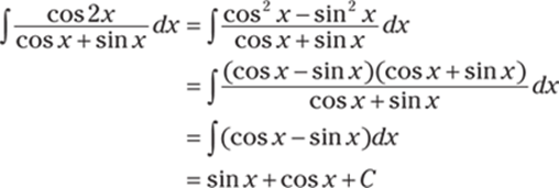
609. –cot x – 2x + C
Begin by using a trigonometric identity on the numerator of the integrand. Then split up the fraction and rewrite both fractions using trigonometric identities:
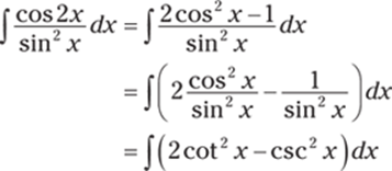
Notice that the first term of the integrand does not have an elementary antiderivative, so you can use a trigonometric identity again to simplify and then integrate:
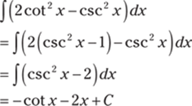
610. sin x + C
Begin by factoring cos x from the numerator and use a trigonometric identity to simplify:
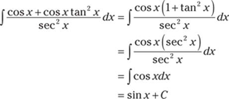
611. the net change in the baby's weight in pounds during the first 2 weeks of life
The net change theorem states that the integral of a rate of change is the net change:
![]()
Because w'(t) is the rate of the baby's growth in pounds per week, w(t) represents the child's weight in pounds at age t. From the net change theorem, you have
![]()
Therefore, the integral represents the increase in the child's weight (in pounds) from birth to the start of the second week.
612. the total amount of oil, in gallons, that leaks from the tanker for the first 180 minutes after the leak begins.
Because r(t) is the rate at which oil leaks from a tanker in gallons per minute, you can write r(t) = –V'(t), where V(t) is the volume of the oil at time t. Notice that you need the minus sign because the volume is decreasing, so V'(t) is negative but r(t) is positive. By the net change theorem, you have
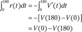
This is the number of gallons of oil that leaks from the tank in the first 180 minutes after the leak begins.
613. the total bird population 6 months after they're placed in the refuge
Because p'(t) is the rate of growth of the bird population per month, p(t) represents the bird population after t months. From the net change theorem, you have
![]()
This represents the change in the bird population in 6 months. Therefore, ![]() represents the total bird population after 6 months.
represents the total bird population after 6 months.
614. the net change of the particle's position, or displacement, during the first 10 seconds
Because s'(t) = v(t), where s(t) is the position function of the particle after t seconds, you have
![]()
This represents the net change of the particle's position, or displacement, during the first 10 seconds. Notice that because the velocity is in meters per second, the displacement units are in meters.
615. the net change in the car's velocity, in meters per second, from the end of the third second to the end of the fifth second
Because v'(t) = a(t), where v(t) is the velocity function of the car after t seconds, you have
![]()
This represents the net change in the car's velocity, in meters per second, from the end of the third second to the end of the fifth second.
616. the total number of solar panels produced from the end of the second week to the end of the fourth week
Because P'(t) is the rate of production per week, P(t) represents the total number of solar panels produced after t weeks. By the net change theorem, you have
![]()
This represents the total number of solar panels produced from the end of the second week to the end of the fourth week.
617. the net change in the charge from time t1 to time t2
I(t) is defined as the derivative of the charge, Q'(t) = I(t), so by the net change theorem, you have
![]()
This represents the net change in the charge from time t1 to time t2.
618. the net change in income in dollars during the first 10 years at the job
I(t) = I'(t), where I(t) represents your total income after t years, so by the net change theorem, you have
![]()
This represents the net change in income in dollars during the first 10 years at the job.
619. the net change in the amount of water in the pool from the end of the 60th minute to the end of the 120th minute
Because w'(t) is the rate at which water enters the pool in gallons per minute, w(t) represents the amount of water in the pool at time t. By the net change theorem, you have
![]()
This represents the net change in the amount of water in the pool from the end of the 60th minute to the end of the 120th minute.
620. 5
Note that displacement, or change in position, can be positive or negative or zero. You can think of the particle moving to the left if the displacement is negative and moving to the right if the displacement is positive.
Velocity is the rate of change in displacement with respect to time, so if you integrate the velocity function over an interval where the velocity is negative, you're finding how far the particle travels to the left over that time interval (the value of the integral is negative to indicate that the displacement is to the left). Likewise, if you integrate the velocity function over an interval where the velocity is positive, you're finding the distance that the particle travels to the right over that time interval (in this case, the value of the integral is positive). By combining these two values — that is, by integrating the velocity function over the given time interval — you find the net displacement.
To find the displacement, simply integrate the velocity function over the given interval:
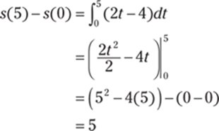
621. ![]()
To find the displacement, simply integrate the velocity function over the given interval:
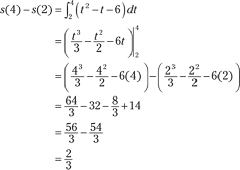
622. 0
To find the displacement, simply integrate the velocity function over the given interval:
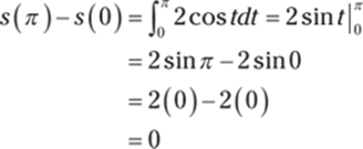
623. ![]()
To find the displacement, simply integrate the velocity function over the given interval:
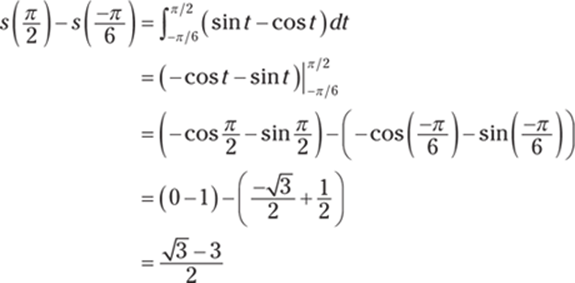
624. ![]()
To find the displacement, simply integrate the velocity function over the given interval:
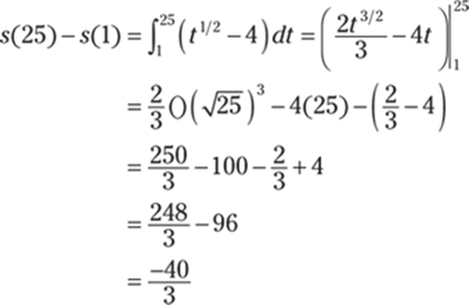
625. 13
Note that displacement, or change in position, can be positive or negative or zero. You can think of the particle moving to the left if the displacement is negative and moving to the right if the displacement is positive.
Velocity is the rate of change in displacement with respect to time, so if you integrate the velocity function over an interval where the velocity is negative, you're finding how far the particle travels to the left over that time interval (the value of the integral is negative to indicate that the displacement is to the left). Likewise, if you integrate the velocity function over an interval where the velocity is positive, you're finding the distance that the particle travels to the right over that time interval (in this case, the value of the integral is positive). By combining these two values, you find the net displacement.
Unlike displacement, distance can't be negative. In order to find the distance traveled, you can integrate the absolute value of the velocity function because you're then integrating a function that's greater than or equal to zero on the given interval.
![]()
Find any zeros of the function on the given interval so you can determine where the velocity function is positive or negative. In this case, you have 2t – 4 = 0 so that t = 2. Because the velocity function is negative on the interval (0, 2) and positive on the interval (2, 5), the distance traveled is
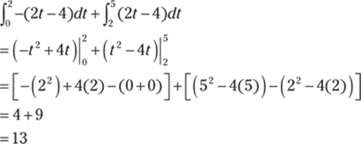
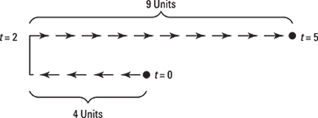
626. 5
Unlike displacement, distance can't be negative. In order to find the distance traveled, you can integrate the absolute value of the velocity function because you're then integrating a function that's greater than or equal to zero on the given interval.
![]()
Find any zeros of the function on the given interval so you can determine where the velocity function is positive or negative. In this case, you have t2 – t – 6 = 0, or (t – 3)(t + 2) = 0, which has solutions t = 3 and t = –2. Because the velocity function is negative on the interval (2, 3) and positive on the interval (3, 4), the distance traveled is

627. 4
Unlike displacement, distance can't be negative. In order to find the distance traveled, you can integrate the absolute value of the velocity function because you're then integrating a function that's greater than or equal to zero on the given interval.
![]()
Find any zeros of the function on the given interval so you can determine where the velocity function is positive or negative. In this case, you have 2 cos t ≥ 0 on ![]() and 2 cos t ≤ 0 on
and 2 cos t ≤ 0 on ![]() . Therefore, the distance traveled is
. Therefore, the distance traveled is
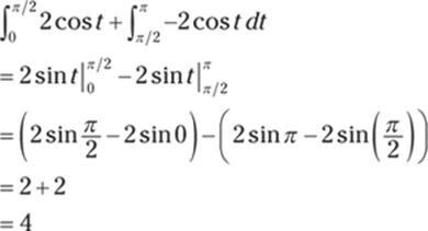
628. ![]()
Unlike displacement, distance can't be negative. In order to find the distance traveled, you can integrate the absolute value of the velocity function because you're then integrating a function that's greater than or equal to zero on the given interval.
![]()
Find any zeros of the function on the given interval so you can determine where the velocity function is positive or negative. In this case, you have sin t – cos t = 0 so that sin t = cos t, which has a solution ![]() on the given interval. Note that on the interval
on the given interval. Note that on the interval ![]() , you have sint – cos t < 0 and that on the interval
, you have sint – cos t < 0 and that on the interval ![]() , sin t – cos t > 0. Therefore, the distance traveled is
, sin t – cos t > 0. Therefore, the distance traveled is
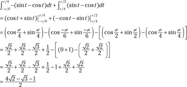
629. ![]()
Unlike displacement, distance can't be negative. In order to find the distance traveled, you can integrate the absolute value of the velocity function because you're then integrating a function that's greater than or equal to zero on the given interval.
![]()
Find the any zeros of the function on the given interval so you can determine where the velocity function is positive or negative. In this case, you have ![]() so that
so that ![]() , or t = 16. Notice that on the interval (1, 16), you have
, or t = 16. Notice that on the interval (1, 16), you have ![]() , whereas on the interval (16, 25), you have
, whereas on the interval (16, 25), you have ![]() . Therefore, the distance traveled is
. Therefore, the distance traveled is
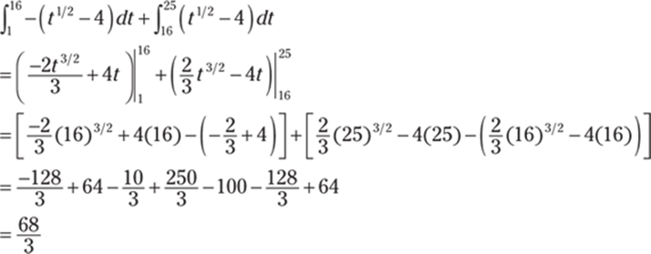
630. ![]()
Because the derivative of the position function is the rate of change in position with respect to time, the derivative of the position function gives you the velocity function. Likewise, the derivative of the velocity function is the rate of change in velocity with respect to time, so the derivative of the velocity function gives you the acceleration function. It follows that the antiderivative of the acceleration function is the velocity function and that the antiderivative of the velocity function is the position function.
First find the velocity function by evaluating the antiderivative of the acceleration function, a(t) = t + 2:

Next, use the initial condition, v(0) = –6, to solve for the arbitrary constant of integration:
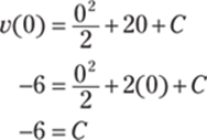
Therefore, the velocity function is
![]()
To find the displacement, simply integrate the velocity function over the given interval, 0 ≤ t ≤ 8:
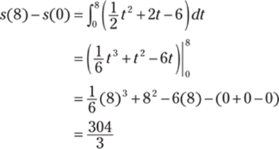
631. ![]()
First find the velocity function by evaluating the antiderivative of the acceleration function, a (t) = 2t + 1:

Next, use the initial condition, v (0) = –12, to solve for the arbitrary constant of integration:

Therefore, the velocity function is
![]()
Next, find the displacement by integrating the velocity function over the given interval, 0 ≤ t ≤ 5:
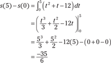
632. ![]()
First find the velocity function by evaluating the antiderivative of the acceleration function, a (t) = sin t + cos t:

Next, use the initial condition, ![]() , to solve for the arbitrary constant of integration:
, to solve for the arbitrary constant of integration:
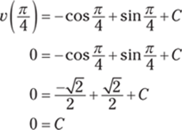
Therefore, the velocity function is
![]()
Next, find the displacement by integrating the velocity function over the given interval, ![]() :
:
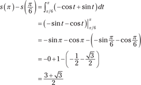
633. ![]()
Because the derivative of the position function is the rate of change in position with respect to time, the derivative of the position function gives you the velocity function. Likewise, the derivative of the velocity function is the rate of change in velocity with respect to time, so the derivative of the velocity function gives you the acceleration function. It follows that the antiderivative of the acceleration function is the velocity function and that the antiderivative of the velocity function is the position function.
Note that displacement, or change in position, can be positive or negative or zero. You can think of the particle moving to the left if the displacement is negative and moving to the right if the displacement is positive. But unlike displacement, distance can't be negative. To find the distance traveled, you can integrate the absolute value of the velocity function because you're then integrating a function that's greater than or equal to zero on the given interval.
Begin by finding the velocity function by evaluating the antiderivative of the acceleration function, a(t) = t + 2:

Next, use the initial condition, v(0) = –6, to solve for the arbitrary constant of integration:

Therefore, the velocity function is
![]()
To find the distance traveled, integrate the absolute value of the velocity function over the given interval:

Find any zeros of the function on the given interval so that you can determine where the velocity function is positive or negative: ![]() , or t2 + 4t – 12 = 0, which factors as (t + 6)(t – 2) = 0 and has the solutions of t = –6, t = 2. Notice that on the interval (0, 2), the velocity function is negative and that on the interval (2, 8), the velocity function is positive. Therefore, the distance traveled is
, or t2 + 4t – 12 = 0, which factors as (t + 6)(t – 2) = 0 and has the solutions of t = –6, t = 2. Notice that on the interval (0, 2), the velocity function is negative and that on the interval (2, 8), the velocity function is positive. Therefore, the distance traveled is
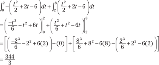
634. ![]()
Begin by finding the velocity function by evaluating the antiderivative of the acceleration function, a (t) = 2t + 1:

Next, use the initial condition, v (0) = –12, to solve for the arbitrary constant of integration:

Therefore, the velocity function is
![]()
To find the distance traveled, integrate the absolute value of the velocity function over the given interval:
![]()
Find any zeros of the function on the given interval so you can determine where the velocity function is positive or negative: t2 + t – 12 = 0 factors as (t + 4)(t – 3) = 0 and has the solutions t = –4, t = 3. The velocity function is negative on the interval (0, 3) and positive on the interval (3, 5), so the distance traveled is
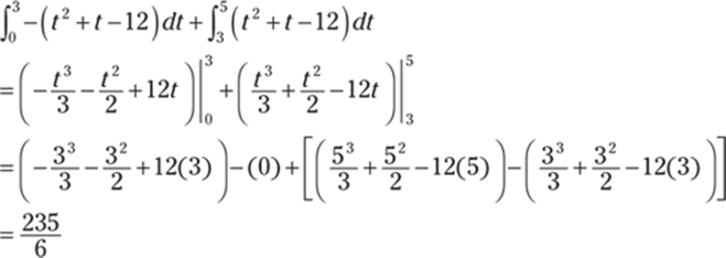
635. ![]()
Begin by finding the velocity function by evaluating the antiderivative of the acceleration function, a (t) = sin t + cos t:

Next, use the initial condition, ![]() , to solve for the arbitrary constant of integration:
, to solve for the arbitrary constant of integration:
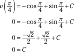
Therefore, the velocity function is
![]()
To find the distance traveled, integrate the absolute value of the velocity function over the given interval, ![]() :
:
![]()
Find any zeros of the velocity function on the given interval so you can determine where the velocity function is positive or negative:
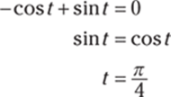
The velocity function is negative on the interval ![]() and positive on the interval
and positive on the interval ![]() , so the total distance traveled is
, so the total distance traveled is

636. ![]()
Recall that the area A of the region bounded by the curves y = f (x) and y = g(x) and by the lines x = a and x = b, where f and g are continuous and f (x) ≥ g(x) for all x in [a, b], is
![]()
More generically, in terms of a graph, you can think of the formula as
![]()
Note that lines x = a and x = b may not be given, so the limits of integration often correspond to points of intersection of the functions.
Begin by finding the points of intersection by setting the functions equal to each other and solving for x:
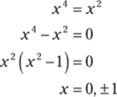
Because x2 ≥ x4 on the interval [–1, 1], the integral to find the area is
![]()
The integrand is an even function, so it's symmetric about the y-axis; therefore, you can instead integrate on the interval [0, 1] and multiply by 2:
![]()
This gives you the following:

The following figure shows the region bounded by the given curves:
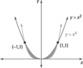
637. ![]()
Begin by finding the points of intersection by setting the functions equal to each other and solving for x:
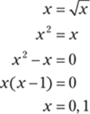
To determine which function is larger on the interval (0, 1), take a point inside the interval and substitute it into each function. If you use ![]() , then the first curve gives you
, then the first curve gives you ![]() , and the second curve gives you
, and the second curve gives you ![]() . Therefore,
. Therefore, ![]() on (0, 1). That means the integral for the area of the bounded region is
on (0, 1). That means the integral for the area of the bounded region is
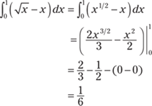
638. ![]()
Because cos x + 1 ≥ x on [0, 1], the integral to find the area is
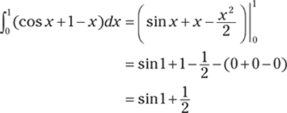
639. ![]()
Recall that the area A of the region bounded by the curves x = f (y) and x = g(y) and by the lines y = a and y = b, where f and g are continuous and f (y) ≥ g(y) for all y in [a, b], is
![]()
More generically, in terms of a graph, you can think of the formula as
![]()
Note that lines y = a and y = b may not be given, so the limits of integration often correspond to points of intersection of the curves.
In this case, you could integrate with respect to x, but you'd have to solve each equation for y by completing the square, which would needlessly complicate the problem.
Begin by finding the points of intersection by setting the expressions equal to each other and solving for y:
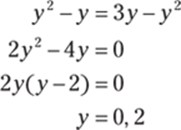
To determine which function has larger x values for y in the interval (0, 2), pick a point in the interval and substitute it into each function. So if y = 1, then x = 12 – 1 = 0 and x = 3(1) – 12 = 2. Therefore, the integral to find the area is
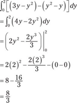
640. ![]()
In this case, you can easily solve the two equations for x, so integrating with respect to y makes sense. If you instead solved the equations for y, you'd have to use more than one integral when integrating with respect to x to set up the area.
Begin by solving the first equation for x to get x = y2 – 1. Because ![]() on the interval [0, 1], the integral to find the area is
on the interval [0, 1], the integral to find the area is
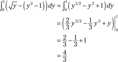
641. ![]()
Notice that you can easily solve the two equations for x, so integrating with respect to y makes sense. If you were to solve the first equation for y in order to integrate with respect to x, you'd have to use more than one integral to set up the area.
Begin by solving the second equation for x to get x = y + 7. Then find the points of intersection by setting the expressions equal to each other and solving for y:
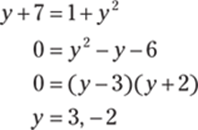
To determine which curve has the larger x values for y on the interval (–2, 3), pick a point in the interval and substitute it into each equation. If y = 0, then x = 1 + 02 = 1 and x = 0 + 7 = 7. Therefore, the integral to find the area is
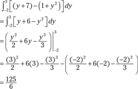
The following figure shows the region bounded by the given curves:
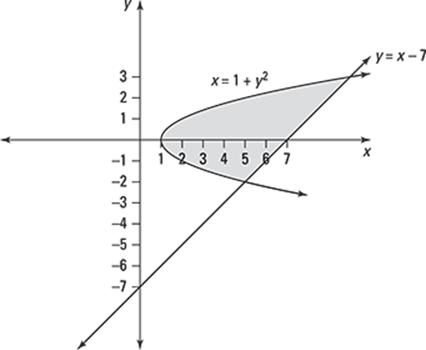
642. ![]()
Begin by finding the point of intersection of the two curves by setting them equal to each other and solving for y:
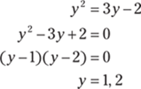
Notice that 3y – 2 > y2 for y in the interval (1, 2). Therefore, the integral to find the area of the region is
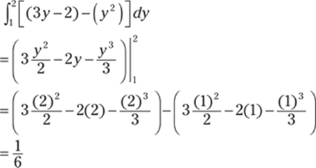
643. ![]()
In this case, integrating with respect to y makes sense. You could integrate with respect to x, but you'd have to solve x = 2y2 for y and then use two integrals to compute the area, because the “top function” isn't the same for the entire region.
Begin by isolating x in the second equation to get x = 1 – y. Then find the points of intersection by setting the expressions equal to each other and solving for y:
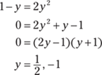
To determine which curve has the larger x values for y in the interval ![]() , pick a point in the interval and substitute it into each equation. So if y = 0, then x = 2(0)2 = 0 and x + 0 = 1. Therefore, x = 1 – y is the rightmost curve and x = 2y2 is the leftmost curve, which means the integral to find the area is
, pick a point in the interval and substitute it into each equation. So if y = 0, then x = 2(0)2 = 0 and x + 0 = 1. Therefore, x = 1 – y is the rightmost curve and x = 2y2 is the leftmost curve, which means the integral to find the area is
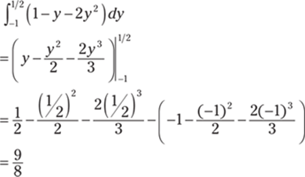
The following figure shows the region bounded by the given curves:
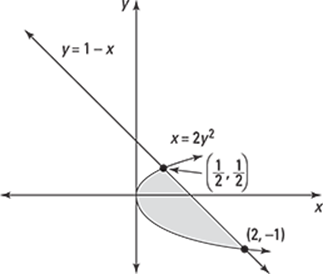
644. 36
Begin by finding the points of intersection by setting the functions equal to each other and solving for x:
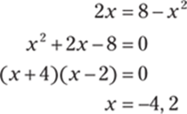
To determine which function is larger on the interval (–4, 2), take a point inside the interval and substitute it into each function. If you let x = 0, then y = 2(0) = 0 and y = 8 – 02 = 8. Therefore, 8 – x2 > 2x on (–4, 2), so the integral for the area of the bounded region is
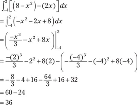
The following figure shows the region bounded by the given curves:
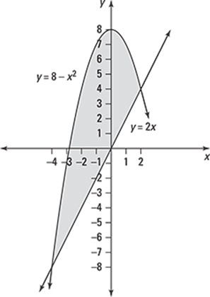
645. ![]()
In this example, integrating with respect to y makes sense. You could integrate with respect to x, but you'd have to solve both x = 2 – y2 and x = y2 – 2 for y and then use two integrals to compute the area, because the “top function” and the “bottom function” aren't the same for the entire region. (You could actually reduce the region to a single integral by using symmetry, but that isn't possible in general.)
Begin by finding the points of intersection by setting the expressions equal to each other and solving for y:
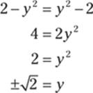
To determine which curve has the larger x values for y in the interval ![]() , take a point inside the interval and substitute it into each function. So if y = 0, then x = 2 – 02 = 2 and x = 02 – 2 = –2; therefore, 2 – y2 > y2 – 2 on
, take a point inside the interval and substitute it into each function. So if y = 0, then x = 2 – 02 = 2 and x = 02 – 2 = –2; therefore, 2 – y2 > y2 – 2 on ![]() . That means the integral to find the area is
. That means the integral to find the area is
![]()
By symmetry, you can rewrite the integral as
![]()
Now you can evaluate the integral:
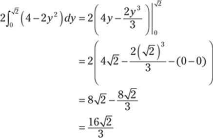
The following figure shows the region bounded by the given curves:
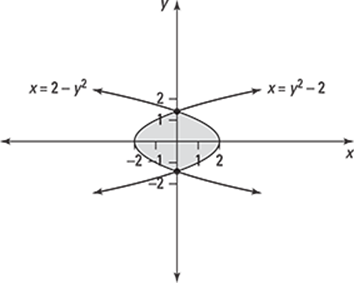
646. 72
Begin by finding the points of intersection by setting the functions equal to each other and solving for x:
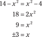
To determine which function is larger on the interval (–3, 3), take a point inside the interval and substitute into each function. If x = 0, then y = 14 – 02 = 14 and y = 02 – 4 = –4. Therefore, 14 – x2 > x2 on the interval (–3, 3), so the integral for the area of the bounded region becomes
![]()
The integrand is an even function, so it's symmetric about the y-axis; therefore, you can instead integrate on the interval [0, 3] and multiply by 2:
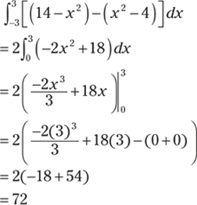
647. ![]()
In this example, integrating with respect to y makes sense. You could integrate with respect to x, but you'd have to solve 4x + y2 = –3 for y and then use two integrals to compute the area, because the “top function” isn't the same for the entire region.
Begin by solving the second equation for x to get ![]() . To find the points of intersection, set the expressions equal to each other and solve for y:
. To find the points of intersection, set the expressions equal to each other and solve for y:
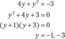
To determine which curve has larger x values for y in the interval (–3, 1), pick a point inside the interval and substitute it into each function. So if y = –2, then x = –2 and ![]() . Therefore, the integral to find the area is
. Therefore, the integral to find the area is
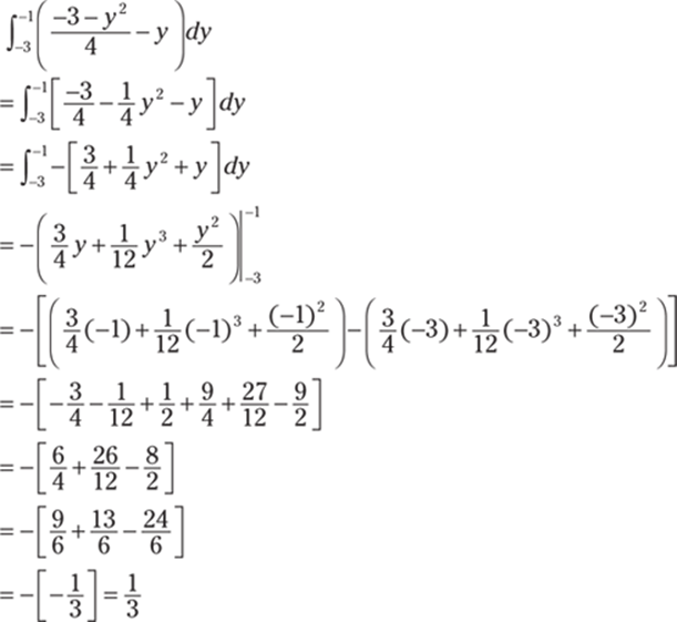
648. ![]()
Begin by finding the points of intersection of the two curves by setting them equal to each other and solving for y:
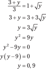
To determine which curve has the larger x values for y on the interval (0, 9), pick a value in the interval and substitute it into each equation. So if y = 1, then ![]() and
and ![]() . Therefore, the integral to find the area is
. Therefore, the integral to find the area is
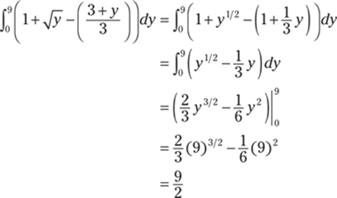
649. ![]()
Notice that the functions ![]() and y = cos x intersect when
and y = cos x intersect when ![]() . On the interval
. On the interval ![]() , you have
, you have ![]() , and on the interval
, and on the interval ![]() , you have
, you have ![]() . Therefore, the integrals to find the area of the region are
. Therefore, the integrals to find the area of the region are
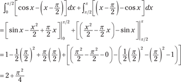
650. ![]()
Begin by finding the points of intersection by setting the functions equal to each other and solving for x:
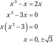
To determine which function is larger on the interval ![]() , take a point in the interval and substitute it into each function to determine which is larger. If x = –1, then y = (–1)3 – (–1) = 0 and y = 2(–1) = –2; therefore, x3 – x > 2x on
, take a point in the interval and substitute it into each function to determine which is larger. If x = –1, then y = (–1)3 – (–1) = 0 and y = 2(–1) = –2; therefore, x3 – x > 2x on ![]() . In a similar manner, check which function is larger on the interval
. In a similar manner, check which function is larger on the interval ![]() . By letting x = 1, you can show that 2x > x3 – x on
. By letting x = 1, you can show that 2x > x3 – x on ![]() . Therefore, the integral to find the area of the region is
. Therefore, the integral to find the area of the region is
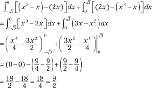
The following figure shows the region bounded by the given curves:
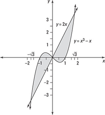
651. ![]()
Notice that you can easily solve the two equations for x, so integrating with respect to y makes sense. If you were to solve the second equation for y in order to integrate with respect to x, you'd have to use more than one integral to set up the area.
Solve the first equation for x to get x = –y. Then find the points of intersection by setting the equations equal to each other and solving for y:
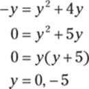
To determine which curve has larger x values on the interval (–5, 0), pick a point in the interval and substitute it into each equation. If y = –1, then x = –(–1) = 1 and x = (–1)2 + 4(–1) = –3. Therefore, the integral to find the area is
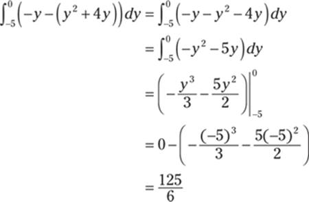
652. ![]()
Begin by setting the expressions equal to each other and solving for y to find the points of intersection:
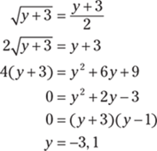
To determine which curve has larger x values for y on the interval (–3, 1), take a point in the interval and substitute it into each equation. So if y = –2, then ![]() and
and ![]() . Therefore, the integral to find the area of the region is
. Therefore, the integral to find the area of the region is
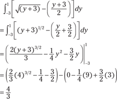
653. ![]()
Begin by finding the point of intersection on the interval ![]() by setting the functions equal to each other and solving for x: sin x = cos x has a solution when
by setting the functions equal to each other and solving for x: sin x = cos x has a solution when ![]() .
.
To determine which function is larger on each interval, pick a point in the interval and substitute it into each function. On the interval ![]() , you have cos x ≥ sin x, and on the interval
, you have cos x ≥ sin x, and on the interval ![]() , you have sin x ≥ cos x. Therefore, the integrals required to find the area of the region are
, you have sin x ≥ cos x. Therefore, the integrals required to find the area of the region are
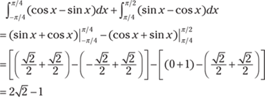
The following figure shows the region bounded by the functions.
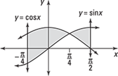
654. ![]()
Begin by finding the points of intersection of the two curves by setting the expressions equal to each other and solving for y:
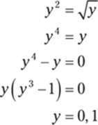
To determine which expression has larger x values for y on the interval (0, 1), pick a point in the interval and substitute it into each equation. So if ![]() , then
, then  and
and ![]() . For y on the interval (0, 1), you have
. For y on the interval (0, 1), you have ![]() . Similarly, you can show that
. Similarly, you can show that ![]() for y on the interval (1, 2). Therefore, the integrals to find the area of the region are
for y on the interval (1, 2). Therefore, the integrals to find the area of the region are
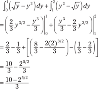
655. ![]()
Begin by finding the points of intersection of the two curves by setting the expressions equal to each other:
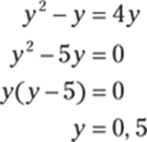
To determine which curve has the larger x values for y on the interval (0, 5), take a point in the interval and substitute it into each equation. So if y = 1, then x = 12 – 1 = 0 and x = 4(1) = 4. Therefore, the integral to find the area of the region is
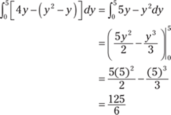
656. 18
Notice that you can easily solve the two equations for x, so integrating with respect to y makes sense. If you were to solve the second equation for y in order to integrate with respect to x, you'd have to complete the square to solve for y, which would needlessly complicate the problem.
Begin by solving both equations for x to get ![]() and x = y + 1. Then set the expressions equal to each other and solve for y to find the points of intersection:
and x = y + 1. Then set the expressions equal to each other and solve for y to find the points of intersection:
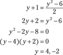
To find which curve has the larger x values for y on the interval (–2, 4), take a point in the interval and substitute it into each equation. So if y = 0, then ![]() and x = 0 + 1 = 1. Therefore, the integral to find the area of the region is
and x = 0 + 1 = 1. Therefore, the integral to find the area of the region is
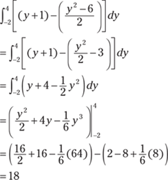
657. ![]()
Begin by finding all the points of intersection of the three functions. To do so, solve each equation for y and then set the functions equal to each other. Solving the second equation for y gives you ![]() , and solving the third equation for y gives you y = 3 – 2x. Set these two functions equal to each other and solve for x:
, and solving the third equation for y gives you y = 3 – 2x. Set these two functions equal to each other and solve for x:
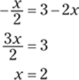
Likewise, finding the other points of intersection gives you ![]() so that x = 0 is a solution and gives you x = 3 – 2x so that x = 1 is a solution.
so that x = 0 is a solution and gives you x = 3 – 2x so that x = 1 is a solution.
Notice that on the interval (0, 1), the region is bounded above by the function y = x and below by the function ![]() . On the interval (1, 2), the region is bounded above by the function y = 3 – 2x and below by the function
. On the interval (1, 2), the region is bounded above by the function y = 3 – 2x and below by the function ![]() . Therefore, the integrals to find the area of the region are
. Therefore, the integrals to find the area of the region are
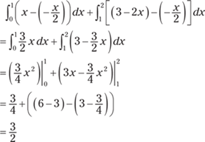
658. ![]()
Begin by finding the points of intersection by setting the functions equal to each other. Square both sides of the equation and factor to solve for x:
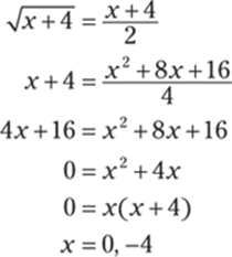
To determine which function is larger on the interval (–4, 0), pick a point inside the interval and substitute it into each equation. So if x = –3, then ![]() and
and ![]() . Because
. Because ![]() on (–4, 0), the integral to find the area is
on (–4, 0), the integral to find the area is
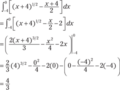
659. 18
To find the points of intersection, begin by noting that ![]() on the interval [0, ∞). To find the point of intersection on [0, 8), set the functions equal to each other and solve for x:
on the interval [0, ∞). To find the point of intersection on [0, 8), set the functions equal to each other and solve for x:
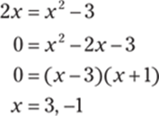
Because the interval under consideration is [0, 8), use the solution x = 3.
Likewise, on (–∞, 0), you have ![]() . Again, find the point of intersection by setting the functions equal to each other and solving for x:
. Again, find the point of intersection by setting the functions equal to each other and solving for x:
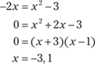
Because the interval under consideration is (–∞, 0), keep only the solution x = –3. (You could have also noted that because both ![]() and y = x2 – 3 are even functions, then if there's a point of intersection at x = 3, there must also be a point of intersection at x = –3.)
and y = x2 – 3 are even functions, then if there's a point of intersection at x = 3, there must also be a point of intersection at x = –3.)
On the interval (–3, 3), you have ![]() . Therefore, the integral to find the area is
. Therefore, the integral to find the area is
![]()
By symmetry, you can rewrite the integral as
![]()
Finally, simplify and evaluate this integral:
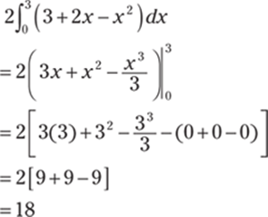
The following figure shows the region bounded by the given curves:
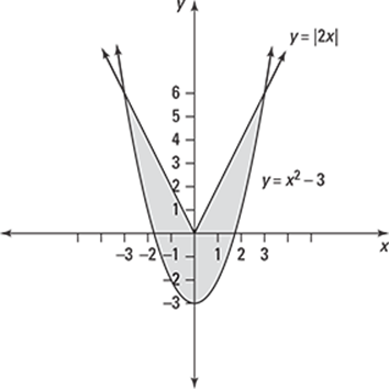
660. ![]()
Begin by finding the points of intersection on the interval ![]() by setting the functions equal to each other:
by setting the functions equal to each other:
![]()
Use an identity on the right-hand side of the equation and factor:

Now set each factor equal to zero and solve for x: cos x = 0 and 2 sin x – 1 = 0, or ![]() . On the interval
. On the interval ![]() , you have cos x = 0 if
, you have cos x = 0 if ![]() and
and ![]() if
if ![]() . On the interval
. On the interval ![]() , you have cos x > sin(2x), and on
, you have cos x > sin(2x), and on ![]() , you have sin(2x) > cos x. Therefore, the integrals to find the area are
, you have sin(2x) > cos x. Therefore, the integrals to find the area are
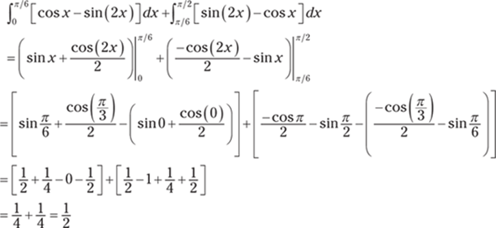
The following figure shows the region bounded by the given curves:
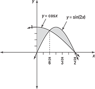
661. ![]()
Begin by finding the point of intersection by setting the functions y = 2e2x and y = 3 – 5ex equal to each other and solving for x:
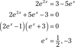
Because ex = –3 has no solution, the only solution is ![]() . Note that
. Note that ![]() , so the line x = 0 bounds the region on the right so that the upper limit of integration is b = 0.
, so the line x = 0 bounds the region on the right so that the upper limit of integration is b = 0.
To determine which function is larger on the interval  , pick a point inside the interval and substitute it into each equation. On the interval
  , notice that 2e2x > 5ex. Therefore, the integral to find the area is
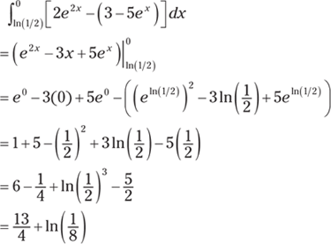
662. ![]()
Recall the definition of volume: Let S be a solid that lies between x = a and x = b. If A(x) is the cross-sectional area of S in the plane Px that goes through x and is perpendicular to the x-axis, where A is a continuous function, then the volume of S is
![]()
Here's the region that's being rotated. Because the cross-sectional slice is a circle, you have A(x) = π(y)2 = π(f (x))2.
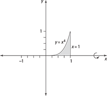
Note that when y = 0, you have 0 = x4 so that x = 0 is the lower limit of integration.
The integral to find the volume is
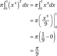
663. 2π
Recall the definition of volume: Let S be a solid that lies between y = c and y = d. If A(y) is the cross-sectional area of S in the plane Py that goes through y and is perpendicular to the y-axis, where A is a continuous function, then the volume of S is
![]()
Here's the region that's being rotated. Because the cross-sectional slice is a circle, you have A(y) = π(x)2 = π(g(y))2.
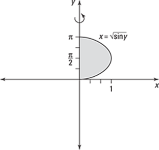
In this case, the limits of integration correspond to y = 0 and y = π. Because ![]() , the integral to find the area becomes
, the integral to find the area becomes
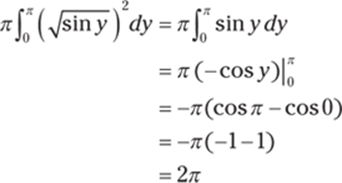
664. ![]()
Recall the definition of volume: Let S be a solid that lies between x = a and x = b. If A(x) is the cross-sectional area of S in the plane Px that goes through x and is perpendicular to the x-axis, where A is a continuous function, then the volume of S is
![]()
Because the cross-sectional slice is a circle in this case, you have A(x) = π(y)2 = π(f (x))2. Here, the limits of integration correspond to the lines x = 3 and x = 5. Because ![]() , the integral to find the volume is
, the integral to find the volume is
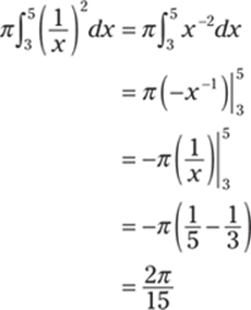
665. π ln 3
Recall the definition of volume: Let S be a solid that lies between x = a and x = b. If A(x) is the cross-sectional area of S in the plane Px that goes through x and is perpendicular to the x-axis, where A is a continuous function, then the volume of S is
![]()
Because the cross-sectional slice is a circle in this case, you have A(x) = π(y)2 = π(f (x))2. Here, the limits of integration correspond to the lines x = 1 and x = 3. Because ![]() , the integral to find the volume is
, the integral to find the volume is
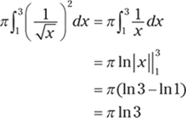
666. π
Recall the definition of volume: Let S be a solid that lies between x = a and x = b. If A(x) is the cross-sectional area of S in the plane Px that goes through x and is perpendicular to the x-axis, where A is a continuous function, then the volume of S is
![]()
Here's the region that's being rotated. Because the cross-sectional slice is a circle, you have A(x) = π(y)2 = π(f (x))2.
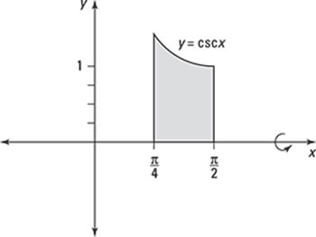
In this case, the limits of integration correspond to the lines ![]() and
and ![]() . Because y = csc x, the integral to find the volume is
. Because y = csc x, the integral to find the volume is
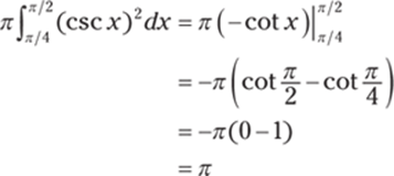
667. ![]()
Recall the definition of volume: Let S be a solid that lies between x = a and x = b. If A(x) is the cross-sectional area of S in the plane Px that goes through x and is perpendicular to the x-axis, where A is a continuous function, then the volume of S is
![]()
Because the cross-sectional slice is a circle in this case, you have A(x) = π(y)2 = π(f (x))2.
Begin by isolating y in the first equation:

If you let y = 0 in this equation, you get x = 4, which corresponds to the upper limit of integration. Therefore, you have the following integral:
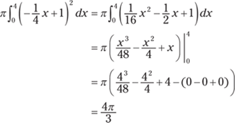
668. ![]()
Recall the definition of volume: Let S be a solid that lies between y = c and y = d. If A(y) is the cross-sectional area of S in the plane Py that goes through y and is perpendicular to the y-axis, where A is a continuous function, then the volume of S is
![]()
Here's the region that's being rotated. Because the cross-sectional slice is a circle, you have A(y) = π(x)2 = π(g(y))2.
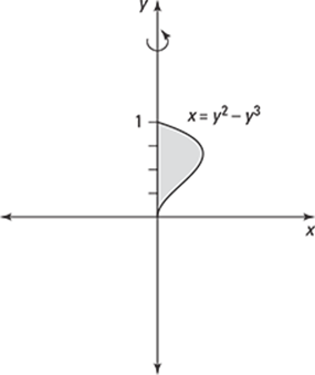
Begin by setting the expressions equal to each other and solving for y in order to find the limits of integration:

Therefore, the integral to find the volume is
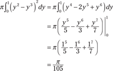
669. 8π
Recall the definition of volume: Let S be a solid that lies between x = a and x = b. If A(x) is the cross-sectional area of S in the plane Px that goes through x and is perpendicular to the x-axis, where A is a continuous function, then the volume of S is
![]()
Because the cross-sectional slice is a circle in this case, you have A(x) = π(y)2 = π(f (x))2.
To get the lower limit of integration, find where the function ![]() intersects the line y = 0. Set the equations equal to each other and solve for x:
intersects the line y = 0. Set the equations equal to each other and solve for x:

Therefore, x = 1 and x = 5 are the limits of integration. Because ![]() , the integral becomes
, the integral becomes
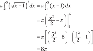
670. ![]()
Recall the definition of volume: Let S be a solid that lies between x = a and x = b. If A(x) is the cross-sectional area of S in the plane Px that goes through x and is perpendicular to the x-axis, where A is a continuous function, then the volume of S is
![]()
In this case, the cross-sectional slice has the shape of a washer. When the cross-sectional slice is a washer, you can find A(x) by using

where the outer radius, rout, is the distance of the function farther away from the line of rotation and the inner radius, rin, is the distance of the function closer to the line of rotation at a particular value of x.
First find the limits of integration by finding the points of intersection of the two curves. Set the functions equal to each other and solve for x:
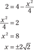
On the interval ![]() , you have
, you have ![]() so that
so that ![]() and rin = 2. Therefore, the integral to find the volume is
and rin = 2. Therefore, the integral to find the volume is
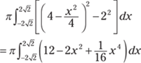
Notice that ![]() is an even function, so it's symmetric about the y-axis. Therefore, you can instead make zero the lower limit of integration and double the value of the integral:
is an even function, so it's symmetric about the y-axis. Therefore, you can instead make zero the lower limit of integration and double the value of the integral:
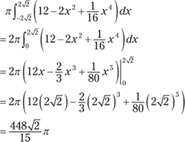
671. ![]()
Recall the definition of volume: Let S be a solid that lies between y = c and y = d. If A(y) is the cross-sectional area of S in the plane Py that goes through y and is perpendicular to the y-axis, where A is a continuous function, then the volume of S is
![]()
Because the cross-sectional slice is a circle in this case, you have A(y) = π(x)2 = π(g(y))2.
Note that y = 8 gives you one of the limits of integration; find the other limit of integration by setting the functions equal to each other and solving for y:

With the limits of integration y = 0 and y = 8 and with g(y) = y2/3, the volume of the region is
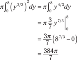
672. ![]()
Recall the definition of volume: Let S be a solid that lies between x = a and x = b. If A(x) is the cross-sectional area of S in the plane Px that goes through x and is perpendicular to the x-axis, where A is a continuous function, then the volume of S is
![]()
Because the cross-sectional slice is a circle in this case, you have A(x) = π(y)2 = π(f (x))2.
Notice that ![]() intersects y = 0 when x = r and when x = –r, which corresponds to the limits of integration. Therefore, the integral to find the volume becomes
intersects y = 0 when x = r and when x = –r, which corresponds to the limits of integration. Therefore, the integral to find the volume becomes
![]()
Because y = r2 – x2 is an even function, you can change the lower limit of integration to zero and multiply by 2 to evaluate the integral:
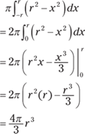
By rotating the semicircular region, you've found the formula for the volume of a sphere!
673. ![]()
Recall the definition of volume: Let S be a solid that lies between x = a and x = b. If A(x) is the cross-sectional area of S in the plane Px that goes through x and is perpendicular to the x-axis, where A is a continuous function, then the volume of S is
![]()
Here's the region that's being rotated:
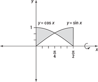
In this case, the cross-sectional slice has the shape of a washer. When the cross-sectional slice is a washer, you can find A(x) by using

where the outer radius, rout, is the distance of the function farther away from the line of rotation and the inner radius, rin, is the distance of the function closer to the line of rotation at a particular value of x.
Begin by finding the point of intersection of the two functions by setting them equal to each other: sin x = cos x, which has the solution ![]() on the interval
on the interval ![]() . Notice that on the interval
. Notice that on the interval ![]() , you have cos x > sin x so that rout = cos x and rin = sin x, and on the interval
, you have cos x > sin x so that rout = cos x and rin = sin x, and on the interval ![]() , you have sin x > cos x so that rout = sin x and rin = sin x. Therefore, the integrals to find the volume are
, you have sin x > cos x so that rout = sin x and rin = sin x. Therefore, the integrals to find the volume are
![]()
Because ![]() and
and ![]() are equal, you can compute the volume by evaluating the integral on the interval
are equal, you can compute the volume by evaluating the integral on the interval ![]() and doubling the answer:
and doubling the answer:
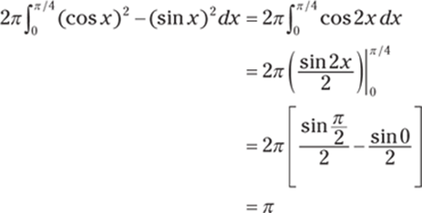
674. ![]()
Recall the definition of volume: Let S be a solid that lies between x = a and x = b. If A(x) is the cross-sectional area of S in the plane Px that goes through x and is perpendicular to the x-axis, where A is a continuous function, then the volume of S is
![]()
Here's the region that's being rotated. Because the cross-sectional slice is a circle, you have A(x) = π(y)2 = π(f (x))2.
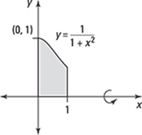
Because the function is bounded by x = 0 and x = 1, these are the limits of integration. With ![]() , the integral to find the volume becomes
, the integral to find the volume becomes

Now use the trigonometric substitution x = tan θ so that dx = sec2 θ dθ. Find the new limits of integration by noting that if x = 1, then 1 = tan θ so that ![]() . Likewise, if x = 0, then 0 = tan θ so that 0 = θ. Using these new values, you produce the following integral:
. Likewise, if x = 0, then 0 = tan θ so that 0 = θ. Using these new values, you produce the following integral:

Now use the identity ![]() =
= ![]() :
:
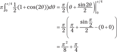
675. ![]()
Recall the definition of volume: Let S be a solid that lies between x = a and x = b. If A(x) is the cross-sectional area of S in the plane Px that goes through x and is perpendicular to the x-axis, where A is a continuous function, then the volume of S is
![]()
In this case, the cross-sectional slice has the shape of a washer. When the cross-sectional slice is a washer, you can find A(x) by using

where the outer radius, rout, is the distance of the function farther away from the line of rotation and the inner radius, rin, is the distance of the function closer to the line of rotation at a particular value of x.
Begin by finding the points of intersection in order to find the limits of integration. Solve the second equation for y, set the expressions equal to each other, and solve for x:
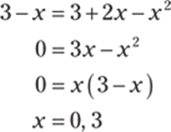
To find out which function is greater on the interval (0, 3) without graphing (and is therefore farther away from the line of rotation), take a point in this interval and substitute that value into each function. So if x = 1, you have y = 3 + 2 – 12 = 4 and y = 3 – 1 = 2. Therefore, rout = 3 + 2x – x2 and rin = 3 – x, so the integral becomes
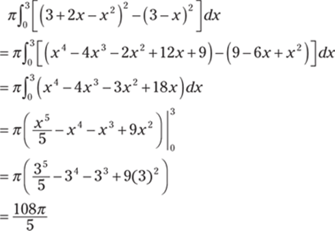
676. ![]()
Recall the definition of volume: Let S be a solid that lies between y = c and y = d. If A(y) is the cross-sectional area of S in the plane Py that goes through y and is perpendicular to the y-axis, where A is a continuous function, then the volume of S is
![]()
In this case, the cross-sectional slice has the shape of a washer. When the cross-sectional slice is a washer, you can find A(y) by using

where the outer radius, rout, is the distance of the expression farther away from the line of rotation and the inner radius, rin, is the distance of the expression closer to the line of rotation at a particular value of y.
The region is being rotated about the line the y-axis, so solve the first equation for x:
![]()
Note that you keep the positive root because the region being rotated is in the first quadrant.
Find the limits of integration by setting the functions equal to each other and solving for y:
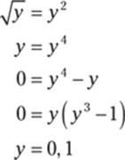
For a value in the interval (0, 1), you have ![]() so that
so that ![]() and
and ![]() . Therefore, the integral to find the volume becomes
. Therefore, the integral to find the volume becomes
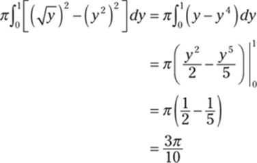
677. ![]()
Recall the definition of volume: Let S be a solid that lies between x = a and x = b. If A(x) is the cross-sectional area of S in the plane Px that goes through x and is perpendicular to the x-axis, where A is a continuous function, then the volume of S is
![]()
Here's the region being rotated:
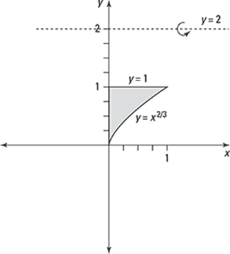
In this case, the cross-sectional slice has the shape of a washer. When the cross-sectional slice is a washer, you can find A(x) by using

where the outer radius, rout, is the distance of the function farther away from the line of rotation and the inner radius, rin, is the distance of the function closer to the line of rotation at a particular value of x.
Begin by finding the point of intersection by setting the functions equal to each other and solving for x:

The limits of integration are therefore x = 0 (given) and x = 1. Note that rout = 2 – x2/3 and rin = 2 – 1 = 1 because you're rotating the region about the line y = 2. Therefore, the integral to find the volume is
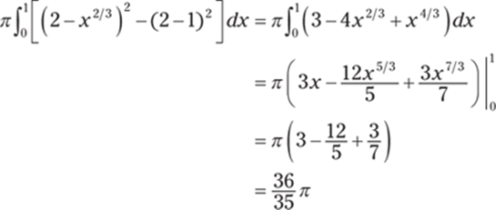
678. ![]()
Recall the definition of volume: Let S be a solid that lies between y = c and y = d. If A(y) is the cross-sectional area of S in the plane Py that goes through y and is perpendicular to the y-axis, where A is a continuous function, then the volume of S is
![]()
In this case, the cross-sectional slice has the shape of a washer. When the cross-sectional slice is a washer, you can find A(y) by using

where the outer radius, rout, is the distance of the expression farther away from the line of rotation and the inner radius, rin, is the distance of the expression closer to the line of rotation at a particular value of y.
At x = 0, you have y = 02/3 = 0, which will be the lower limit of integration; y = 1 corresponds to the upper limit of integration.
Solving the equation y = x2/3 for x gives you x = y3/2. Note that because you're rotating the region about the line x = –1, you have rout = y3/2 + 1 and rin = 0 + 1 = 1. Therefore, the integral to find the volume is
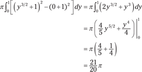
679. ![]()
Recall the definition of volume: Let S be a solid that lies between x = a and x = b. If A(x) is the cross-sectional area of S in the plane Px that goes through x and is perpendicular to the x-axis, where A is a continuous function, then the volume of S is
![]()
Here's the region being rotated:
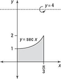
In this case, the cross-sectional slice has the shape of a washer. When the cross-sectional slice is a washer, you can find A(x) by using

where the outer radius, rout, is the distance of the function farther away from the line of rotation and the inner radius, rin, is the distance of the function closer to the line of rotation at a particular value of x.
On the interval ![]() , you have sec x < 4. Because you're rotating the region about the line y = 4, you have rout = 4 and rin = 4 – sec x. Therefore, the integral to find the volume is
, you have sec x < 4. Because you're rotating the region about the line y = 4, you have rout = 4 and rin = 4 – sec x. Therefore, the integral to find the volume is
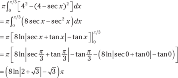
680. ![]()
Recall the definition of volume: Let S be a solid that lies between y = c and y = d. If A(y) is the cross-sectional area of S in the plane Py that goes through y and is perpendicular to the y-axis, where A is a continuous function, then the volume of S is
![]()
In this case, the cross-sectional slice has the shape of a washer. When the cross-sectional slice is a washer, you can find A(y) by using

where the outer radius, rout, is the distance of the expression farther away from the line of rotation and the inner radius, rin, is the distance of the expression closer to the line of rotation at a particular value of y.
Begin by setting the expressions equal to each other to find the points of intersection, which correspond to the limits of integration:

Because you're rotating the region about the line x = 5, you have rout = 5 – y2 and rin = 5 – 4 = 1. Therefore, the integral to find the volume is
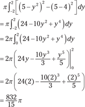
681. 
Recall the definition of volume: Let S be a solid that lies between x = a and x = b. If A(x) is the cross-sectional area of S in the plane Px that goes through x and is perpendicular to the x-axis, where A is a continuous function, then the volume of S is
![]()
Here's the region that's being rotated:
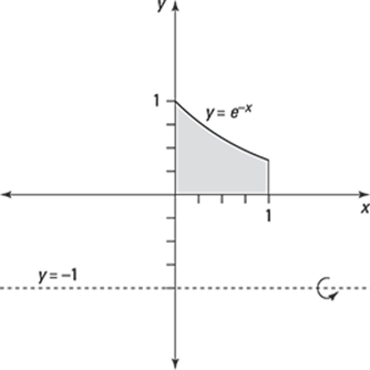
In this case, the cross-sectional slice has the shape of a washer. When the cross-sectional slice is a washer, you can find A(x) by using

where the outer radius, rout, is the distance of the function farther away from the line of rotation and the inner radius, rin, is the distance of the function closer to the line of rotation at a particular value of x.
Note that the lines x = 0 and x = 1 correspond to the limits of integration. Because you're rotating the region about the line y = –1, you have rout = e–x + 1 and rin = 0 + 1 = 1. Therefore, the integral to find the volume becomes
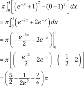
682. ![]()
Recall the definition of volume: Let S be a solid that lies between x = a and x = b. If A(x) is the cross-sectional area of S in the plane Px that goes through x and is perpendicular to the x-axis, where A is a continuous function, then the volume of S is
![]()
Here, you want to find an expression for A(x).
The base is a circle that has a radius of 4 and is centered at the origin, so the equation of the circle is x2 + y2 = 16.

If you consider a cross-sectional slice at point (x, y) on the circle, where y > 0, the base of the square equals 2y; therefore, the area of the cross-sectional slice is (2y)2 = 4y2.
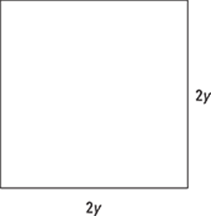
In order to integrate with respect to x, you can solve the equation of the circle for y2 and write the area as 4y2 = 4(16 – x2) = A(x). Because the base of the solid varies for x over the interval [–4, 4], the limits of integration are –4 and 4. Therefore, the integral to find the volume is
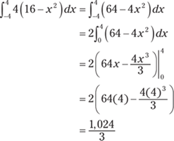
683. ![]()
Recall the definition of volume: Let S be a solid that lies between x = a and x = b. If A(x) is the cross-sectional area of S in the plane Px that goes through x and is perpendicular to the x-axis, where A is a continuous function, then the volume of S is
![]()
Here, you want to find an expression for A(x).
The base is a circle that has a radius of 4 and is centered at the origin, so the equation of the circle is x2 + y2 = 16.
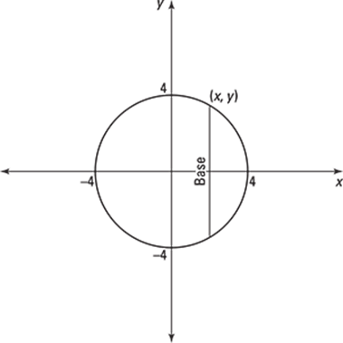
If you consider a cross-sectional slice at point (x, y) on the circle, where y > 0, the base of the equilateral triangle equals 2y and has a height of ![]() ; therefore, the area of the triangle is
; therefore, the area of the triangle is ![]() .
.
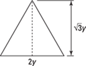
In order to integrate with respect to x, you can solve the equation of the circle for y2 and write the area as ![]() = A(x). Because the base of the solid varies for x over the interval [–4, 4], the limits of integration are –4 and 4. Therefore, the integral to find the volume is
= A(x). Because the base of the solid varies for x over the interval [–4, 4], the limits of integration are –4 and 4. Therefore, the integral to find the volume is
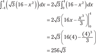
684. 96
Recall the definition of volume: Let S be a solid that lies between y = c and y = d. If A(y) is the cross-sectional area of S in the plane Py that goes through y and is perpendicular to the y-axis, where A is a continuous function, then the volume of S is
![]()
Here, you want to find an expression for A(y).
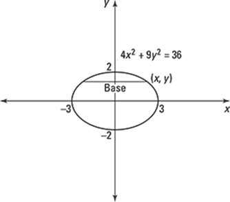
If you consider a cross-sectional slice that goes through a point (x, y) on the ellipse, where x > 0, then one side of the square has length 2x. The area of the square is
![]()
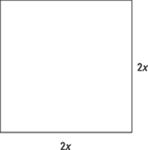
Because the base of the solid varies for y over the interval [–2, 2] the limits of integration are –2 and 2. Therefore, the integral to find the volume is
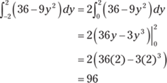
Note that because 36 – 9y2 is an even function of y, the lower limit of integration was changed to zero and the resulting integral was multiplied by 2 to make the integral a bit easier to compute.
685. ![]()
Recall the definition of volume: Let S be a solid that lies between y = c and y = d. If A(y) is the cross-sectional area of S in the plane Py that goes through y and is perpendicular to the y-axis, where A is a continuous function, then the volume of S is
![]()
Here, you want to find an expression for A(y).
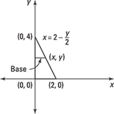
The base of S is the region bounded by the curves x = 0, y = 0, and ![]() . If you consider a cross-sectional slice that goes through a point (x, y) on the line
. If you consider a cross-sectional slice that goes through a point (x, y) on the line ![]() , the cross-sectional slice is an isosceles triangle with height equal to the base, so the area is
, the cross-sectional slice is an isosceles triangle with height equal to the base, so the area is

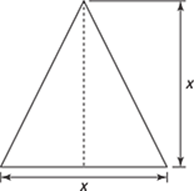
Because the base of the solid varies for y over the interval [0, 4], the limits of integration are 0 and 4. Therefore, the integral to find the volume is
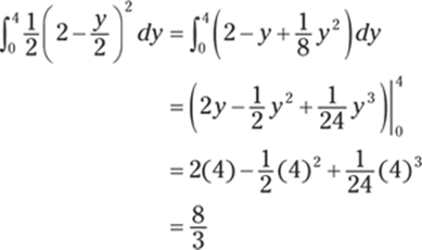
686. 16
Recall the definition of volume: Let S be a solid that lies between x = a and x = b. If A(x) is the cross-sectional area of S in the plane Px that goes through x and is perpendicular to the x-axis, where A is a continuous function, then the volume of S is
![]()
Here, you want to find an expression for A(x).
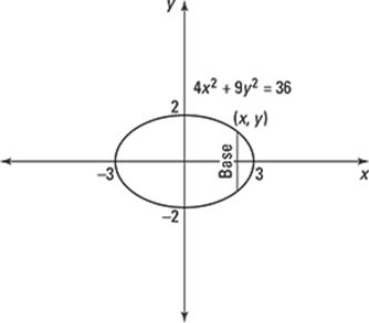
If you consider a cross-sectional slice that goes through a point (x, y) on the ellipse, where y > 0, then the hypotenuse of the right triangle has length 2y. If l is a leg of the isosceles right triangle, then by the Pythagorean theorem, l2 + l2 = (2y)2 so that l2 = 2y2. Solving the elliptical boundary function for y2 gives you ![]() . Therefore, the area of the triangle is
. Therefore, the area of the triangle is
![]()

Because the base of the solid varies for x over the interval [–3, 3], the limits of integration are –3 and 3. Therefore, the integral to find the volume is
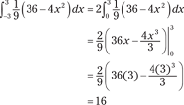
Note that because y = 36 – 4x2 is an even function, the lower limit of integration was changed to zero and the resulting integral was multiplied by 2 to make the integral a bit easier to compute.
687. ![]()
Recall the definition of volume: Let S be a solid that lies between y = c and y = d. If A(y) is the cross-sectional area of S in the plane Py that goes through y and is perpendicular to the y-axis, where A is a continuous function, then the volume of S is
![]()
Here, you want to find an expression for A(y).
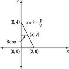
The base of S is the region bounded by the curves x = 0, y = 0, and ![]() . If you consider a cross-sectional slice that goes through a point (x, y) on the line
. If you consider a cross-sectional slice that goes through a point (x, y) on the line ![]() , that cross-sectional slice is a semicircle with a radius of
, that cross-sectional slice is a semicircle with a radius of ![]() . That means the area of the slice is
. That means the area of the slice is


Because the base of the solid varies for y over the interval [0, 4], the limits of integration are 0 and 4. Therefore, the integral to find the volume is
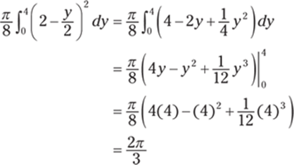
688. 4π
To find the volume of a solid obtained by rotating about the y-axis a region that's under the curve y = f (x) and above the x-axis from x = a to x = b with cylindrical shells, use the integral
![]()
More generically, you can use the formula
![]()
To find the shell radius, let x be in the interval [a, b]; the shell radius is the distance from x to the line of rotation. To find the shell height, let f (x) be the function that bounds the region above and let g(x) be the function that bounds the region below; the shell height is given by f (x) – g(x). Note that the limits of integration often correspond to points of intersection.
Here, the limits of integration are given as x = 1 and x = 3 and the shell height is ![]() , so the integral becomes
, so the integral becomes
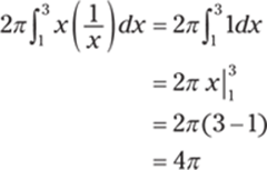
689. 8π
To find the volume of a solid obtained by rotating about the y-axis a region that's under the curve y = f (x) and above the x-axis from x = a to x = b with cylindrical shells, use the integral
![]()
More generically, you can use the formula
![]()
To find the shell radius, let x be in the interval [a, b]; the shell radius is the distance from x to the line of rotation. To find the shell height, let f (x) be the function that bounds the region above and let g(x) be the function that bounds the region below; the shell height is given by f(x) – g(x). Note that the limits of integration often correspond to points of intersection.
Find the other limit of integration by determining where y = x2 and y = 0 intersect: x2 = 0 gives you x = 0. The shell height is x2 – 0, so the integral becomes
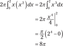
690. ![]()
To find the volume of a solid obtained by rotating about the x-axis a region that's to the left of the curve x = f (y) and to the right of the y-axis from y = c to y = d with cylindrical shells, use the integral
![]()
More generically, you can use the formula
![]()
To find the shell radius, let y be in the interval [c, d]; the shell radius is the distance from y to the line of rotation. To find the shell height, let f (y) be the curve that bounds the region on the right and let g(y) be the curve that bounds the region on the left; the shell height is given by f(y) – g(y). Note that the limits of integration often correspond to points of intersection.
Because y = 1 corresponds to one of the limits of integration, find the other limit of integration by solving the equation 0 = y1/3, which gives you 0 = y. Then find the volume using cylindrical shells:
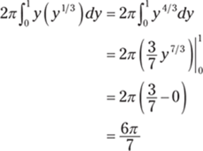
691. ![]()
The region is being rotated about the line x = –1, which is parallel to the y-axis. To find the volume of a solid obtained by rotating about the y-axis a region that's under the curve y = f (x) and above the x-axis from x = a to x = b using cylindrical shells, use the following integral:
![]()
More generically, you can use the formula
![]()
To find the shell radius, let x be in the interval [a, b]; the shell radius is the distance from x to the line of rotation. To find the shell height, let f (x) be the function that bounds the region above and let g(x) be the function that bounds the region below; the shell height is given by f (x) – g(x). Note that the limits of integration often correspond to points of intersection.
The line x = 2 gives you one of the limits of integration, so begin by finding the other limit of integration by determining where the function intersects the x-axis; 0 = x2 gives you 0 = x. Notice that the shell radius is (x + 1), so here's the integral to find the volume using cylindrical shells:
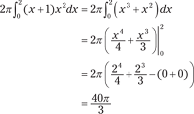
692. 216π
To find the volume of a solid obtained by rotating about the y-axis a region that's under the curve y = f (x) and above the x-axis from x = a to x = b with cylindrical shells, use the integral
![]()
More generically, you can use the formula
![]()
To find the shell radius, let x be in the interval [a, b]; the shell radius is the distance from x to the line of rotation. To find the shell height, let f (x) be the function that bounds the region above and let g(x) be the function that bounds the region below; the shell height is given by f (x) – g(x). Note that the limits of integration often correspond to points of intersection.
Here's the region being rotated about the y-axis:
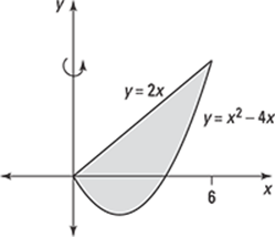
Begin by finding the limits of integration by setting the functions equal to each other and solving for x:
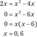
Because 2x ≥ x2 – 4x on the interval [0, 6], the shell height is given by 2x – (x2 – 4x). Therefore, the integral to find the volume is
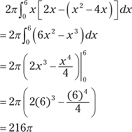
693. ![]()
To find the volume of a solid obtained by rotating about the x-axis a region to the left of the curve x = f (y) and to the right of the y-axis from y = c to y = d with cylindrical shells, use the integral
![]()
More generically, you can use the formula
![]()
To find the shell radius, let y be in the interval [c, d]; the shell radius is the distance from y to the line of rotation. To find the shell height, let f (y) be the curve that bounds the region on the right and let g(y) be the curve that bounds the region on the left; the shell height is given by f(y) – g(y). Note that the limits of integration often correspond to points of intersection.
Begin by isolating the y in the first equation to get y1/4 = x. Find the lower limit of integration by solving y1/4 = 0 to get y = 0. Then find the volume using cylindrical shells:
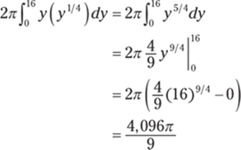
694. ![]()
To find the volume of a solid obtained by rotating about the x-axis a region to the left of the curve x = f (y) and to the right of the y-axis from y = c to y = d with cylindrical shells, use the integral
![]()
More generically, you can use the formula
![]()
To find the shell radius, let y be in the interval [c, d]; the shell radius is the distance from y to the line of rotation. To find the shell height, let f (y) be the curve that bounds the region on the right and let g(y) be the curve that bounds the region on the left; the shell height is given by f(y) – g(y). Note that the limits of integration often correspond to points of intersection.
Here's the region being rotated about the x-axis:
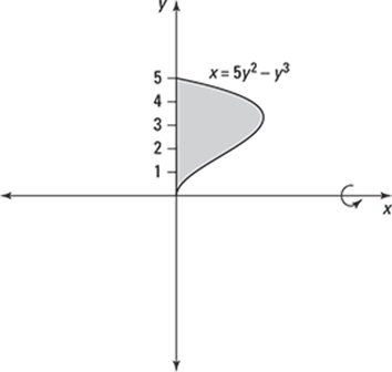
Begin by finding the limits of integration. To do so, find the points of intersection of the two curves by setting the expressions equal to each other and solving for y:

Note that 5y2 – y3 ≥ 0 on the interval [0, 5] so that the shell height is 5y2 – y3 – 0, or simply 5y2 – y3. Therefore, the integral to find the volume is
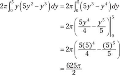
695. 16π
The region is being rotated about the line x = 4, which is parallel to the y-axis. To find the volume of a solid obtained by rotating about the y-axis a region that's under the curve y = f (x) and above the x-axis from x = a to x = b with cylindrical shells, use the integral
![]()
More generically, you can use the formula
![]()
To find the shell radius, let x be in the interval [a, b]; the shell radius is the distance from x to the line of rotation. To find the shell height, let f (x) be the function that bounds the region above and let g(x) be the function that bounds the region below; the shell height is given by f (x) – g(x). Note that the limits of integration often correspond to points of intersection.
Begin by finding the points of intersection by setting the functions equal to each other and solving for x in order to find the limits of integration:
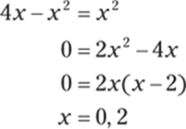
Note that on the interval [0, 2], you have 4x – x2 ≥ x2 so that the shell height is (4x – x2) – (x2). Also note that the region is to the left of the line of rotation x = 4, so the shell radius is (4 – x). Therefore, the integral to find the volume is
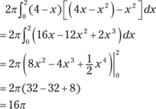
696. ![]()
To find the volume of a solid obtained by rotating about the y-axis a region that's under the curve y = f (x) and above the x-axis from x = a to x = b with cylindrical shells, use the integral
![]()
More generically, you can use the formula
![]()
To find the shell radius, let x be in the interval [a, b]; the shell radius is the distance from x to the line of rotation. To find the shell height, let f (x) be the function that bounds the region above and let g(x) be the function that bounds the region below; the shell height is given by f (x) – g(x). Note that the limits of integration often correspond to points of intersection.
Here, the limits of integration correspond to the lines x = 0 and x = 1, the shell height is (1 + x + x2), and the shell radius is x. Therefore, the integral to find the volume is
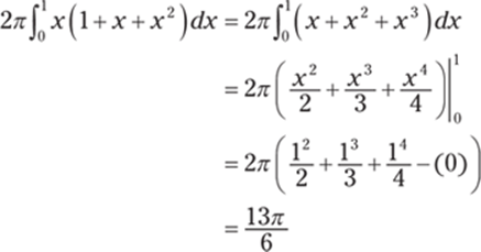
697. ![]()
To find the volume of a solid obtained by rotating about the y-axis a region that's under the curve y = f (x) and above the x-axis from x = a to x = b with cylindrical shells, use the integral
![]()
More generically, you can use the formula
![]()
To find the shell radius, let x be in the interval [a, b]; the shell radius is the distance from x to the line of rotation. To find the shell height, let f (x) be the function that bounds the region above and let g(x) be the function that bounds the region below; the shell height is given by f (x) – g(x). Note that the limits of integration often correspond to points of intersection.
Set the functions equal to each other and solve for x in order to find the other limit of integration:
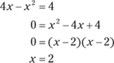
Here, the shell height is given by 4 – (4x – x2) and the shell radius is x, so the integral to find the volume is
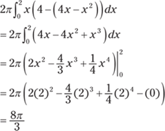
698. ![]()
To find the volume of a solid obtained by rotating about the x-axis a region to the left of the curve x = f (y) and to the right of the y-axis from y = c to y = d with cylindrical shells, use the integral
![]()
More generically, you can use the formula
![]()
To find the shell radius, let y be in the interval [c, d]; the shell radius is the distance from y to the line of rotation. To find the shell height, let f (y) be the curve that bounds the region on the right and let g(y) be the curve that bounds the region on the left; the shell height is given by f(y) – g(y). Note that the limits of integration often correspond to points of intersection.
Notice that if x = 0, then ![]() , so the limits of integration are y = 0 (given) and y = 3. Solving for x in the equation
, so the limits of integration are y = 0 (given) and y = 3. Solving for x in the equation ![]() gives you x = 9 – y2 so that the shell height is (9 – y2). Therefore, the integral to find the volume is
gives you x = 9 – y2 so that the shell height is (9 – y2). Therefore, the integral to find the volume is
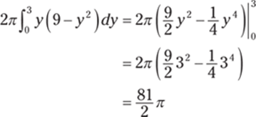
699. ![]()
The region is being rotated about the line x = 2, which is parallel to the y-axis. To find the volume of a solid obtained by rotating about the y-axis a region that's under the curve y = f (x) and above the x-axis from x = a to x = b with cylindrical shells, use the integral
![]()
More generically, you can use the formula
![]()
To find the shell radius, let x be in the interval [a, b]; the shell radius is the distance from x to the line of rotation. To find the shell height, let f (x) be the function that bounds the region above and let g(x) be the function that bounds the region below; the shell height is given by f (x) – g(x). Note that the limits of integration often correspond to points of intersection.
Find the limits of integration by setting the functions equal to each other and solving for x:

Because the line of rotation x = 2 is to the right of the region being rotated, the shell radius is (2 – x). Therefore, to find the volume of revolution using cylindrical shells, you use the following integral:
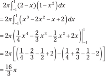
700. ![]()
To find the volume of a solid obtained by rotating about the y-axis a region that's under the curve y = f (x) and above the x-axis from x = a to x = b with cylindrical shells, use the integral
![]()
More generically, you can use the formula
![]()
To find the shell radius, let x be in the interval [a, b]; the shell radius is the distance from x to the line of rotation. To find the shell height, let f (x) be the function that bounds the region above and let g(x) be the function that bounds the region below; the shell height is given by f (x) – g(x). Note that the limits of integration often correspond to points of intersection.
Here's the region being rotated about the y-axis:
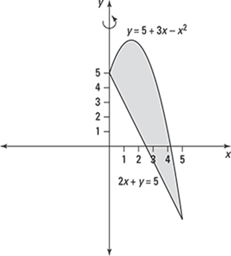
Begin by isolating y in the second equation to get y = 5 – 2x. Then set the expressions equal to each other and solve for x to find the x coordinates of the points of intersection:
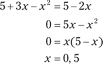
Because 5 + 3x – x2 ≥ 5 – 2x on the interval [0, 5], the shell height is given by (5 + 3x – x2) – (5 – 2x). Therefore, the integral to find the volume is
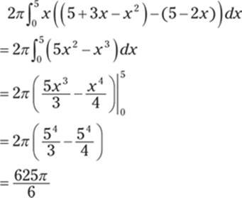
701. ![]()
The region is being rotated about the line x = –1, which is parallel to the y-axis. To find the volume of a solid obtained by rotating about the y-axis a region that's under the curve y = f (x) and above the x-axis from x = a to x = b with cylindrical shells, use the integral
![]()
More generically, you can use the formula
![]()
To find the shell radius, let x be in the interval [a, b]; the shell radius is the distance from x to the line of rotation. To find the shell height, let f (x) be the function that bounds the region above and let g(x) be the function that bounds the region below; the shell height is given by f (x) – g(x). Note that the limits of integration often correspond to points of intersection.
Here's the region being rotated about the line x = –1:
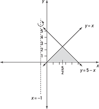
Find the point of intersection using y = x, x + y = 5, and substitution to get x + x = 5 so that ![]() . Notice that on the interval
. Notice that on the interval ![]() , the upper boundary of the region is x and the lower boundary is y = 0; on
, the upper boundary of the region is x and the lower boundary is y = 0; on ![]() the upper boundary of the region is 5 – x and the lower boundary isy = 0. Because the line of rotation is x = –1, the shell radius is (x + 1). Therefore, to find the volume using cylindrical shells, you use two integrals:
the upper boundary of the region is 5 – x and the lower boundary isy = 0. Because the line of rotation is x = –1, the shell radius is (x + 1). Therefore, to find the volume using cylindrical shells, you use two integrals:
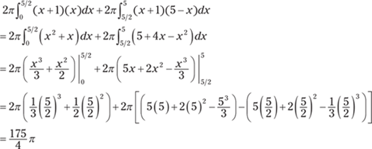
702. 2π
To find the volume of a solid obtained by rotating about the y-axis a region that's under the curve y = f (x) and above the x-axis from x = a to x = b with cylindrical shells, use the integral
![]()
More generically, you can use the formula
![]()
To find the shell radius, let x be in the interval [a, b]; the shell radius is the distance from x to the line of rotation. To find the shell height, let f (x) be the function that bounds the region above and let g(x) be the function that bounds the region below; the shell height is given by f (x) – g(x). Note that the limits of integration often correspond to points of intersection.
In this example, the limits of integration are given as x = 0 and ![]() , and the shell height is sin(x2) – 0, so the integral becomes
, and the shell height is sin(x2) – 0, so the integral becomes
![]()
To evaluate this integral, use the substitution u = x2 so that du = 2 dx, or ![]() . You can find the new limits of integration by noting that if
. You can find the new limits of integration by noting that if ![]() , then
, then ![]() and that if x = 0, then u = 02 = 0. Using these values gives you
and that if x = 0, then u = 02 = 0. Using these values gives you

703. 2π(e2 + 1)
To find the volume of a solid obtained by rotating about the x-axis a region to the left of the curve x = f (y) and to the right of the y-axis from y = c to y = d with cylindrical shells, use the integral
![]()
More generically, you can use the formula
![]()
To find the shell radius, let y be in the interval [c, d]; the shell radius is the distance from y to the line of rotation. To find the shell height, let f (y) be the curve that bounds the region on the right and let g(y) be the curve that bounds the region on the left; the shell height is given by f(y) – g(y). Note that the limits of integration often correspond to points of intersection.
In this example, the limits of integration are given as y = 0 and y = 2, and the shell height is ey – 0. Therefore, to find the volume using cylindrical shells, you use
![]()
To evaluate this integral, use integration by parts with u = y so that du = dy, and let dv = ey dy so that v = ey:
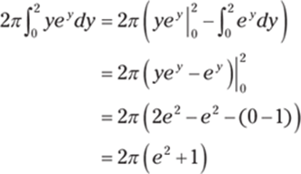
704. 
To find the volume of a solid obtained by rotating about the y-axis a region that's under the curve y = f (x) and above the x-axis from x = a to x = b with cylindrical shells, use the integral
![]()
More generically, you can use the formula
![]()
To find the shell radius, let x be in the interval [a, b]; the shell radius is the distance from x to the line of rotation. To find the shell height, let f (x) be the function that bounds the region above and let g(x) be the function that bounds the region below; the shell height is given by f (x) – g(x). Note that the limits of integration often correspond to points of intersection.
In this example, the limits of integration correspond to the lines x = 0 and x = 3 and the shell height is given by ![]() . Therefore, to find the volume of revolution using cylindrical shells, use the following integral:
. Therefore, to find the volume of revolution using cylindrical shells, use the following integral:
![]()
To evaluate this integral, use the substitution u = –x2 so that du = –2x dx, or ![]() . Find the new limits of integration by noting that if x = 3, then u = –9, and if x = 0, then u = 0. With these new values, the integral becomes
. Find the new limits of integration by noting that if x = 3, then u = –9, and if x = 0, then u = 0. With these new values, the integral becomes
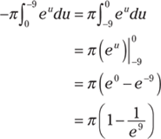
705. ![]()
The region is being rotated about the line x = –1, which is parallel to the y-axis. To find the volume of a solid obtained by rotating about the y-axis a region that's under the curve y = f (x) and above the x-axis from x = a to x = b with cylindrical shells, use the integral
![]()
More generically, you can use the formula
![]()
To find the shell radius, let x be in the interval [a, b]; the shell radius is the distance from x to the line of rotation. To find the shell height, let f (x) be the function that bounds the region above and let g(x) be the function that bounds the region below; the shell height is given by f (x) – g(x). Note that the limits of integration often correspond to points of intersection.
Here's the region being rotated about the line x = –1:
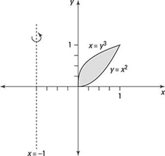
Begin by writing x = y3 as x1/3 = y. Then set the functions equal to each other to find the points of intersection, which give you the limits of integration. Cube both sides of the equation and factor to solve for x:
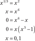
Notice that x1/3 > x2 on the interval [0, 1], so the shell height is (x1/3 – x2). For a value in the interval [0, 1], the distance from x to the line of rotation x = –1 is (x + 1), so the shell radius is (x + 1). Therefore, the integral to find the volume of revolution using cylindrical shells is
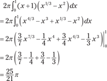
706. 4π(2 ln 3 – 1)
The region is being rotated about the line x = 4, which is parallel to the y-axis. To find the volume of a solid obtained by rotating about the y-axis a region that's under the curve y = f (x) and above the x-axis from x = a to x = b with cylindrical shells, use the integral
![]()
More generically, you can use the formula
![]()
To find the shell radius, let x be in the interval [a, b]; the shell radius is the distance from x to the line of rotation. To find the shell height, let f (x) be the function that bounds the region above and let g(x) be the function that bounds the region below; the shell height is given by f (x) – g(x). Note that the limits of integration often correspond to points of intersection.
Because the region being rotated is to the left of the line of rotation x = 4, the shell radius is (4 – x). To find the volume using cylindrical shells, use the following integral:
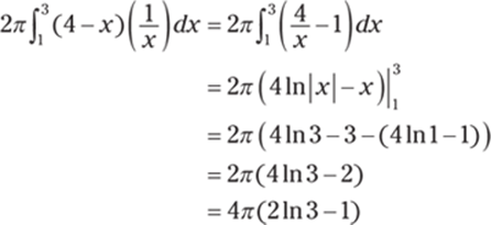
707. ![]()
The region is being rotated about the line y = 1, which is parallel to the x-axis. To find the volume of a solid obtained by rotating about the x-axis a region to the left of the curve x = f (y) and to the right of the y-axis from y = c to y = d with cylindrical shells, use the integral
![]()
More generically, you can use the formula
![]()
To find the shell radius, let y be in the interval [c, d]; the shell radius is the distance from y to the line of rotation. To find the shell height, let f (y) be the curve that bounds the region on the right and let g(y) be the curve that bounds the region on the left; the shell height is given by f(y) – g(y). Note that the limits of integration often correspond to points of intersection.
Here's the region being rotated about the line y = 1:
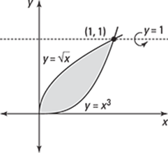
Begin by isolating x in each equation to get y2 = x and y1/3 = x. Set these expressions equal to each other to find the points of intersection, which give you the limits of integration. Cube both sides of the equation and factor to solve for y:
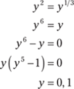
Note that y1/3 > y2 for a point in the interval (0, 1), so the shell height is y1/3 – y2. Also note that the region being rotated is below the line of rotation y = 1, so in the interval (0, 1), the distance from y to the line of rotation is (1 – y), making the shell radius (1 – y). Therefore, the integral to find the volume using cylindrical shells is
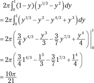
708. ![]()
To find the volume of a solid obtained by rotating about the x-axis a region to the left of the curve x = f (y) and to the right of the y-axis from y = c to y = d with cylindrical shells, use the integral
![]()
More generically, you can use the formula
![]()
To find the shell radius, let y be in the interval [c, d]; the shell radius is the distance from y to the line of rotation. To find the shell height, let f (y) be the curve that bounds the region on the right and let g(y) be the curve that bounds the region on the left; the shell height is given by f(y) – g(y). Note that the limits of integration often correspond to points of intersection.
One of the limits of integration, y = 0, is given. Begin by finding the points of intersection (which will help you find the other limit of integration) by setting the functions equal to each other. Square both sides and factor to solve for x:
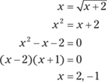
Notice that x = –1 is an extraneous solution. If x = 2, then ![]() , which gives you the other limit of integration.
, which gives you the other limit of integration.
Solving ![]() for x gives you x = y2 – 2. Note that y > y2 – 2 in the interval [0, 2], so the shell height is y – (y2 – 2). Therefore, the integral to find the volume using cylindrical shells is
for x gives you x = y2 – 2. Note that y > y2 – 2 in the interval [0, 2], so the shell height is y – (y2 – 2). Therefore, the integral to find the volume using cylindrical shells is
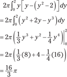
709. 
To find the volume of a solid obtained by rotating about the y-axis a region that's under the curve y = f (x) and above the x-axis from x = a to x = b with cylindrical shells, use the integral
![]()
More generically, you can use the formula
![]()
To find the shell radius, let x be in the interval [a, b]; the shell radius is the distance from x to the line of rotation. To find the shell height, let f (x) be the function that bounds the region above and let g(x) be the function that bounds the region below; the shell height is given by f (x) – g(x). Note that the limits of integration often correspond to points of intersection.
Note that the lines x = 0 and x = 1 correspond to the limits of integration and that the shell height is  , or simply
 ![]() . To find the volume using cylindrical shells, use the following integral:
. To find the volume using cylindrical shells, use the following integral:

Now use the substitution ![]() so that du = –x dx, or –du = x dx. Find the new limits of integration by noting that if x = 1, then
so that du = –x dx, or –du = x dx. Find the new limits of integration by noting that if x = 1, then ![]() , and if x = 0, then u = 0. Using these new values gives you the following:
, and if x = 0, then u = 0. Using these new values gives you the following:
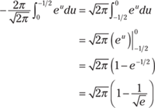
710. 
To find the volume of a solid obtained by rotating about the y-axis a region that's under the curve y = f (x) and above the x-axis from x = a to x = b with cylindrical shells, use the integral
![]()
More generically, you can use the formula
![]()
To find the shell radius, let x be in the interval [a, b]; the shell radius is the distance from x to the line of rotation. To find the shell height, let f (x) be the function that bounds the region above and let g(x) be the function that bounds the region below; the shell height is given by f (x) – g(x). Note that the limits of integration often correspond to points of intersection.
Notice that on the interval [1, 2], you have ![]() , so the shell height is
, so the shell height is ![]() . Therefore, the integral to find the volume is
. Therefore, the integral to find the volume is
![]()
To evaluate ![]() , use integration by parts with u = ln x so that
, use integration by parts with u = ln x so that ![]() , and use dv = x dx so that
, and use dv = x dx so that ![]() . These substitutions give you
. These substitutions give you
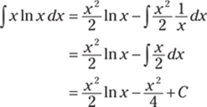
Evaluating the integral ![]() gives you
gives you
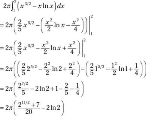
711. π2 – 2π
To find the volume of a solid obtained by rotating about the x-axis a region to the left of the curve x = f (y) and to the right of the y-axis from y = c to y = d with cylindrical shells, use the integral
![]()
More generically, you can use the formula
![]()
To find the shell radius, let y be in the interval [c, d]; the shell radius is the distance from y to the line of rotation. To find the shell height, let f (y) be the curve that bounds the region on the right and let g(y) be the curve that bounds the region on the left; the shell height is given by f(y) – g(y). Note that the limits of integration often correspond to points of intersection.
Here, the limits of integration correspond to the lines y = 0 and ![]() , and the shell height is cos y. To find the volume using cylindrical shells, use the integral
, and the shell height is cos y. To find the volume using cylindrical shells, use the integral
![]()
To evaluate the integral, use integration by parts with u = y so that du = dy, and let dv = cos y dy so that v = sin y:
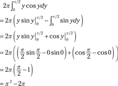
712. 1,470 J
First find the force by multiplying mass by acceleration:
![]()
The force is constant, so no integral is required to find the work:
![]()
713. 9,600 J
The force is constant, so no integral is required to find the work. Enter the numbers in the work equation and solve:
![]()
714. 337.5 ft·lb
Let n be the number of subintervals of length Δx, and let ![]() be a sample point in the
be a sample point in the ![]() subinterval [xi–1, xi].
subinterval [xi–1, xi].
The portion of the rope that is from xi–1 feet to xi feet below the top of the cliff weighs (0.75)Δx pounds and must be lifted approximately ![]() feet. Therefore, its contribution to the total work is approximately
feet. Therefore, its contribution to the total work is approximately ![]() ft·lb. The total work is
ft·lb. The total work is
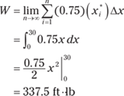
715. 253.125 ft·lb
Let n be the number of subintervals of length Δx, and let ![]() be a sample point in the
be a sample point in the ![]() subinterval [xi–1, xi].
subinterval [xi–1, xi].
First consider the work required to pull the top half of the rope that is from xi–1 feet to xi feet below the top of the cliff, where x is in the interval [0, 15]. This part of the rope weighs (0.75)Δx pounds and must be lifted approximately ![]() feet, so its contribution to the total work is approximately
feet, so its contribution to the total work is approximately ![]() foot-pounds. Therefore, the total work for the top half of the rope is
foot-pounds. Therefore, the total work for the top half of the rope is
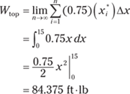
The bottom half of the rope must be lifted 15 feet, so the work required to lift the bottom half is
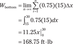
To find the total work required, add the two values: 84.375 + 168.75 = 253.125 ft·lb.
Note that you can find Wbottom without an integral because there's a constant force on this section of the rope!
716. 630,000 ft·lb
Let n be the number of subintervals of length Δx, and let ![]() be a sample point in the
be a sample point in the ![]() subinterval [xi–1, xi].
subinterval [xi–1, xi].
A section of cable that is from xi–1 feet to xi feet below the top of the building weighs 4Δx pounds and must be lifted approximately ![]() feet, so its contribution to the total work is approximately
feet, so its contribution to the total work is approximately ![]() foot-pounds. Therefore, the work required to lift the cable is
foot-pounds. Therefore, the work required to lift the cable is
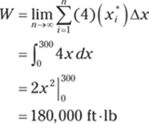
The work required to lift the piece of metal is (1, 500 lb)(300 ft) = 450,000 ft·lb. Therefore, the total work required is 180,000 + 450,000 = 630,000 ft·lb.
717. 22,500 ft·lb
Let n be the number of subintervals of length Δx, and let ![]() be a sample point in the
be a sample point in the ![]() subinterval [xi–1, xi].
subinterval [xi–1, xi].
The cable weighs ![]() . The portion of the cable that is from xi–1 feet to xi feet below the top of the building weighs 2Δx pounds and must be lifted approximately
. The portion of the cable that is from xi–1 feet to xi feet below the top of the building weighs 2Δx pounds and must be lifted approximately ![]() feet, so its contribution to the total work is approximately
feet, so its contribution to the total work is approximately ![]() foot-pounds. The total work is
foot-pounds. The total work is
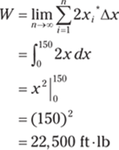
718. 39,200 J
Let n be the number of subintervals of length Δx, and let ![]() be a sample point in the
be a sample point in the ![]() subinterval [xi–1, xi].
subinterval [xi–1, xi].
A horizontal slice of water that is Δx meters thick and is at a distance of ![]() meters from the top of the tank has a volume of ((4)(2)(Δx)) cubic meters and has a mass of
meters from the top of the tank has a volume of ((4)(2)(Δx)) cubic meters and has a mass of

Because mass is not a force, you must multiply it by the acceleration due to gravity, 9.8 meters per second squared, in order to find the weight of the slice in newtons:
![]()
The work required to pump out this slice of water is approximately ![]() joules. Therefore, the total work is
joules. Therefore, the total work is
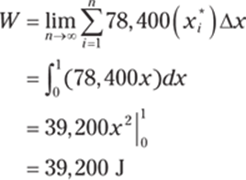
719. 7.875 ft·lb
Begin by finding the spring constant, k, using the information about the work required to stretch the spring 2 feet beyond its natural length:
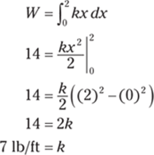
Next, find the work required to stretch the spring 18 inches, or 1.5 feet, beyond its natural length:
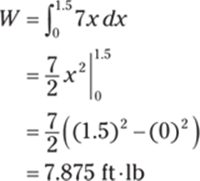
720. 1.51 J
Begin by using the equation F(x) = kx to find the value of the spring constant. Make sure you convert the centimeters to meters so you can use the units newton-meters, or joules.

Now compute the work, again making sure to convert the lengths into meters. Because you're stretching the spring from 12 centimeters beyond its natural length to 22 centimeters beyond its natural length, the limits of integration are from ![]() to
to ![]() ; therefore, the integral to compute the work is
; therefore, the integral to compute the work is
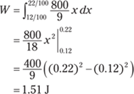
721. ![]()
Use an integral to find the work:
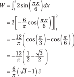
722. 25.2 J
Begin by finding the spring constant, k, using the information about the initial work required to stretch the spring 10 centimeters, or 0.10 meters, from its natural length:
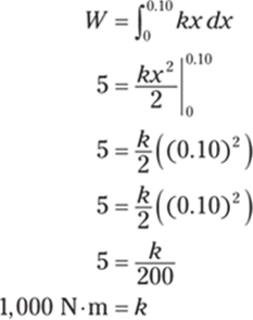
Now find the work required to stretch the spring from 30 centimeters to 42 centimeters, or from 0.15 meters from its natural length to 0.27 meters from its natural length:
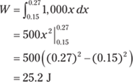
723. ![]()
Begin by using the equation F(x) = kx to find the value of k, the spring constant. The force is measured in foot-pounds, so make sure the length is in feet rather than inches.

Therefore, the force equation is F (x) = 30x.
Because the spring starts at its natural length, x = 0 is the lower limit of integration. Because the spring is stretched 8 inches, or ![]() feet, beyond its natural length, the upper limit of integration is
feet, beyond its natural length, the upper limit of integration is ![]() . Therefore, the integral to find the work is
. Therefore, the integral to find the work is
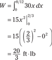
724. 2.25 J
Begin by using the equation F (x) = kx to find the value of the spring constant. Make sure you convert the centimeters to meters so you can use the units newton-meters, or joules. If x is the distance the spring is stretched beyond its natural length, then ![]() . Therefore, the spring constant is
. Therefore, the spring constant is

Now compute the work, making sure to convert the distances into meters. Because you're computing the work while moving the spring from 5 centimeters beyond its natural length to 10 centimeters beyond its natural length, the limits of integration are from ![]() to
to ![]() .
.
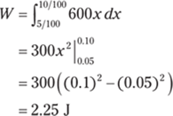
725. 400 ft·lb
Let n be the number of subintervals of length Δx, and let ![]() be a sample point in the ith subinterval [xi–1, xi]. Let
be a sample point in the ith subinterval [xi–1, xi]. Let ![]() be the distance from the middle of the chain.
be the distance from the middle of the chain.
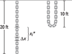
Notice that when you're lifting the end of the chain to the top, only the bottom half of the chain moves. A section of chain that is Δx in length and that is ![]() feet from the middle of the chain weighs 4Δx pounds and will move approximately
feet from the middle of the chain weighs 4Δx pounds and will move approximately ![]() feet. Therefore, the work required is
feet. Therefore, the work required is

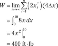
726. 613 J
Let n be the number of subintervals of length Δx, and let ![]() be a sample point in the ith subinterval [xi–1, xi].
be a sample point in the ith subinterval [xi–1, xi].
The part of the chain x meters from the lifted end is raised 5 – x meters if 0 ≤ x ≤ 5 and is lifted 0 meters otherwise. Therefore, the work required is
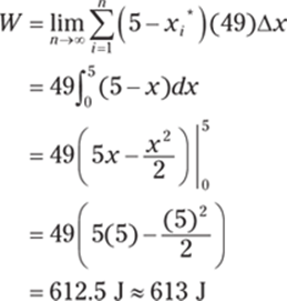
727. 3,397,333 J
Let n be the number of subintervals of length Δx, and let ![]() be a sample point in the ith subinterval [xi–1, xi].
be a sample point in the ith subinterval [xi–1, xi].
Consider a horizontal slice of water that is Δx meters thick and is at a height of ![]() meters from the bottom of the tank. The trough has a triangular face with a width and height of 4 meters, so by similar triangles, the width of the slice of water is the same as the height
meters from the bottom of the tank. The trough has a triangular face with a width and height of 4 meters, so by similar triangles, the width of the slice of water is the same as the height ![]() ; therefore, the volume of the slice of water is
; therefore, the volume of the slice of water is ![]() cubic meters. To find the weight of the water, multiply the acceleration due to gravity (g = 9.8 m/s2) by the mass, which equals the density of water (1,000 kg/m3) multiplied by the volume:
cubic meters. To find the weight of the water, multiply the acceleration due to gravity (g = 9.8 m/s2) by the mass, which equals the density of water (1,000 kg/m3) multiplied by the volume:
![]()
The water must travel a distance of ![]() meters to exit the tank. Therefore, the total work required is
meters to exit the tank. Therefore, the total work required is
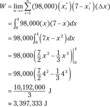
728. 169,646 ft·lb
Let n be the number of subintervals of length Δx, and let ![]() be a sample point in the ith subinterval [xi–1, xi].
be a sample point in the ith subinterval [xi–1, xi].
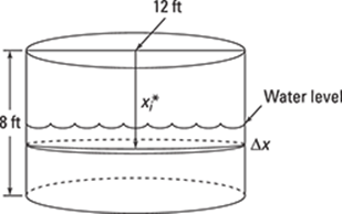
A horizontal slice of water that is Δx feet thick and is at a depth of ![]() feet from the top of the tank is cylindrical, so it has a volume of
feet from the top of the tank is cylindrical, so it has a volume of ![]() cubic feet. Because water weighs 62.5 pounds per cubic foot, this slice of water weighs
cubic feet. Because water weighs 62.5 pounds per cubic foot, this slice of water weighs ![]() pounds. The work required to pump out this slice of water is
pounds. The work required to pump out this slice of water is
![]()
Therefore, the total work is
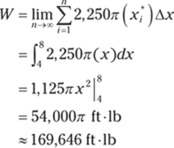
729. 3,000 ft·lb
Let n be the number of subintervals of length Δx, and let ![]() be a sample point in the ith subinterval [xi–1, xi].
be a sample point in the ith subinterval [xi–1, xi].
The work required to lift only the bucket is
![]()
Lifting the bucket takes 50 seconds, so the bucket is losing 1 pound of water per second. At time t (in seconds), the bucket is ![]() feet above the original 100-foot depth, but it now holds only (50 – t) pounds of water. In terms of distance, the bucket holds
feet above the original 100-foot depth, but it now holds only (50 – t) pounds of water. In terms of distance, the bucket holds ![]() pounds of water when it's
pounds of water when it's ![]() feet above the original 100-foot depth. Moving this amount of water a distance of Δx requires
feet above the original 100-foot depth. Moving this amount of water a distance of Δx requires ![]() foot-pounds of work. Therefore, the work required to lift the only the water is
foot-pounds of work. Therefore, the work required to lift the only the water is
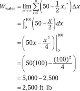
Adding the work to lift the bucket gives you the total work required: 500 + 2,500 = 3,000 foot-pounds.
730. 4 cm
Begin by using the information about how much work is required to stretch the spring from 8 to 10 centimeters to solve for the spring constant and the natural length of the spring; you do so by setting up a system of equations.
You don't know the natural length L for the integral involved in stretching the spring from 8 centimeters to 10 centimeters beyond its natural length, so the limits of integration for one of the integrals involving work are from 0.08 – L to 0.10 – L. Likewise, the other integral will have limits of integration from 0.10 – L to 0.12 – L. Therefore, you have the following two equations for work:
![]()
![]()
Expanding the first of the two integrals gives you
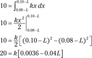
Likewise, expanding the second integral gives you
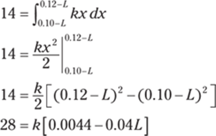
Now solve for the spring constant k. By subtracting 20 = k[0.0036 – 0.04L] from 28 = k[0.0044 – 0.04L], you're left with 8 = k(0.0008) so that k = 10,000.
Finally, find the natural length of the spring. Substituting the value of k into the equation 20 = k[0.0036 – 0.04L] gives you 20 = 10,000[0.0036 – 0.04L], and solving for L yields 0.04 m = L. Therefore, the natural length of the spring is 4 centimeters.
731. 5.29 ft
Let n be the number of subintervals of length Δx, and let ![]() be a sample point in the ith subinterval [xi–1, xi].
be a sample point in the ith subinterval [xi–1, xi].
A horizontal slice of water that is Δx feet thick and is at a distance of ![]() feet from the top of the tank is cylindrical and therefore has a volume of
feet from the top of the tank is cylindrical and therefore has a volume of ![]() cubic feet. Because water weighs 62.5 pounds per cubic foot, this slice of water weighs
cubic feet. Because water weighs 62.5 pounds per cubic foot, this slice of water weighs ![]() pounds. The work required to pump out this slice of water is
pounds. The work required to pump out this slice of water is
![]()
You don't know how many feet of water are pumped out, so you need to solve for the upper limit of integration in the equation:
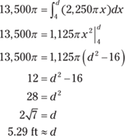
Because the water level in the tank was reduced, the water is now 5.29 feet from the top of the tank.
732. 16.67 cm
Begin by using the information about how much work is required to stretch the spring from 40 to 60 centimeters (0.40 to 0.60 meters) beyond its natural length to solve for the spring constant and the natural length of the spring; to do so, set up a system of equations.
Because you don't know the natural length L for the integral involved in stretching the spring from 0.40 meters to 0.60 meters beyond its natural length, the limits of integration for one of the integrals involving work are from 0.40 – L to 0.60 – L. Likewise, the other integral will have limits of integration from 0.60 – L to 0.80 – L. Therefore, you have the following two equations for work:
![]()
![]()
Expanding the first of the two integrals gives you
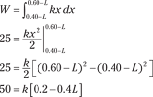
Likewise, expanding the second integral gives you
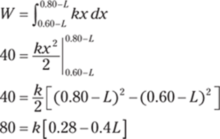
Now solve for the spring constant k. By subtracting 50 = k[0.2 – 0.4L] from 80 = k[0.28 – 0.4L], you're left with 30 = k(0.08) so that k = 375.
Finally, find the natural length of the spring. Substituting the value of k into the equation 50 = k[0.2 – 0.4L] gives you 50 = 375[0.2 – 0.4L]; solving for L yields ![]() meters, so the natural length of the spring is approximately 16.67 centimeters.
meters, so the natural length of the spring is approximately 16.67 centimeters.
733. ![]()
Let n be the number of subintervals of length Δx and let ![]() be a sample point in the ith subinterval.
be a sample point in the ith subinterval.
Here's a view of the tank underground:
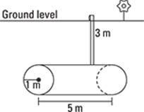
And here's a cross-section of the tank:

A horizontal slice of water that is Δx meters thick and is at a distance of ![]() meters down from the middle of the tank has a volume of
meters down from the middle of the tank has a volume of  cubic meters. To find the weight of the water, multiply the acceleration due to gravity (g = 9.8 m/s2) by the mass of the water, which equals the density of water (1,000 kg/m3) times the volume:

The slice of water must travel a distance of ![]() meters to reach ground level. (Note that negative x values correspond to slices of water that are above the middle of the tank.) Therefore, the total work required is
meters to reach ground level. (Note that negative x values correspond to slices of water that are above the middle of the tank.) Therefore, the total work required is
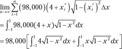
Notice that second integral is zero because ![]() is an odd function being integrated over an interval that's symmetric about the origin. To evaluate
is an odd function being integrated over an interval that's symmetric about the origin. To evaluate ![]() , notice that the integral represents the area of a semicircle with a radius of 1, so the work equals
, notice that the integral represents the area of a semicircle with a radius of 1, so the work equals

734. 20,944 ft·lb
Here's a view of the tank and its cross-section:
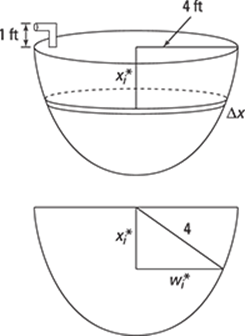
Let n be the number of subintervals of length Δx and let ![]() be a sample point in the ith subinterval. Consider a horizontal slice of water that is Δx feet thick and is at a distance of
be a sample point in the ith subinterval. Consider a horizontal slice of water that is Δx feet thick and is at a distance of ![]() feet from the top of the tank; let
feet from the top of the tank; let ![]() be the radius of the slice of water. Because the tank has a shape of a hemisphere of radius 4, you have the following relationship:
be the radius of the slice of water. Because the tank has a shape of a hemisphere of radius 4, you have the following relationship:
![]()
Therefore, the slice has a volume of
![]()
And the force on this slice is
![]()
The slice of water must travel a distance of ![]() feet to exit the tank. Therefore, the total work required is
feet to exit the tank. Therefore, the total work required is
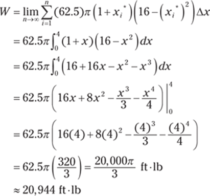
735. 14,726 ft·lb
Here's a view of the tank and its cross-section:
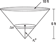
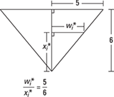
Let n be the number of subintervals of length Δx and let ![]() be a sample point in the ith subinterval. Consider a horizontal slice of water that is Δx feet thick and is
be a sample point in the ith subinterval. Consider a horizontal slice of water that is Δx feet thick and is ![]() feet from the bottom of the tank with a width of
feet from the bottom of the tank with a width of ![]() . This slice has a volume of
. This slice has a volume of
![]()
By similar triangles, you have  , so
, so ![]() ; therefore, the volume becomes
; therefore, the volume becomes
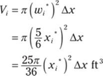
The force on this slice of water is
![]()
The distance this slice must travel to exit the tank is ![]() feet. Therefore, the total work required is
feet. Therefore, the total work required is
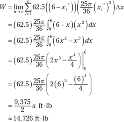
736. ![]()
Using the average value formula with a = –1, b = 2, and f (x) = x3 gives you
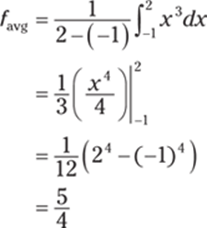
737. ![]()
Using the average value formula with a = 0, ![]() , and f (x) = sin x gives you
, and f (x) = sin x gives you
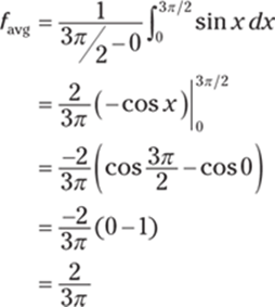
738. ![]()
Using the average value formula with a = 0, ![]() , and f (x) = (sin3 x)(cos x) gives you
, and f (x) = (sin3 x)(cos x) gives you

Next, use the substitution u = sin x so that du = cos x dx. Find the new limits of integration by noting that if ![]() , then
, then ![]() , and if x = 0, then u = sin 0 = 0. With these new values, you get the following:
, and if x = 0, then u = sin 0 = 0. With these new values, you get the following:
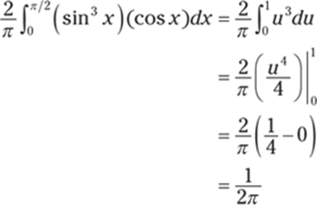
739. ![]()
Using the average value formula with a = 0, b = 2, and ![]() gives you
gives you
![]()
Begin by using the substitution u = 1 + x3 so that du = 3x2 dx, or ![]() . You can also find the new limits of integration by noting that if x = 2, then u = 1 + 23 = 9, and if x = 0, then u = 1 + 03 = 1. With these values, you have the following:
. You can also find the new limits of integration by noting that if x = 2, then u = 1 + 23 = 9, and if x = 0, then u = 1 + 03 = 1. With these values, you have the following:
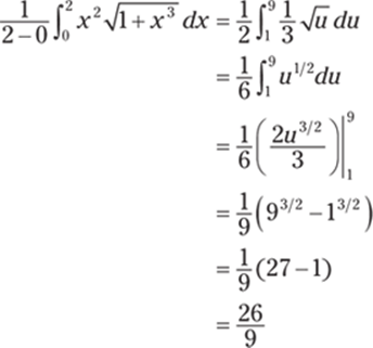
740. ![]()
Using the average value formula with a = 0, b = ln 3, and f (x) = sinh x cosh x, gives you
![]()
Use the substitution u = cosh x so that du = sinh x. You can find the new limits of integration by noting that if x = ln 3, then  , and if x = 0, then
 ![]() . With these new values, you have
. With these new values, you have
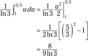
741. ![]()
Using the average value formula with a = 1, b = 4, and  gives you
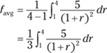
Next, use the substitution u = 1 + r so that du = dr. Find the new limits of integration by noting that if r = 4, then u = 1 + 4 = 5, and if r = 1, then u = 1 + 1 = 2. With these new values, you find that
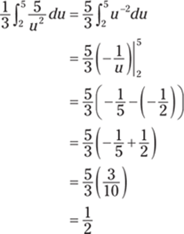
742. ![]()
Using the average value formula with a = 0, b = 8, and ![]() gives you
gives you
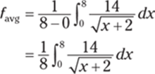
Next, use the substitution u = x + 2 so that du = dx. You can find the new limits of integration by noting that if x = 8, then u = 8 + 2 = 10, and if x = 0, then u = 0 + 2 = 2. With these new values, you find that
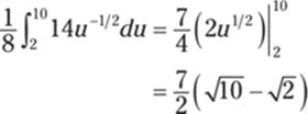
743. d = 1
Using the average value formula with a = 0, b = d, and f (x) = 2 + 4x – 3x2 gives you
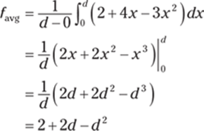
Next, set this expression equal to 3 and solve for d:
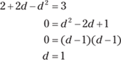
744. d = 4
Using the average value formula with a = 0, b = d, and f (x) = 3 + 6x – 9x2 gives you
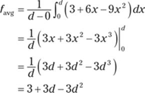
Next, set this expression equal to –33 and solve for d:
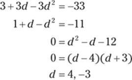
Because the interval is of the form [0, d], the only solution is d = 4.
745. ![]()
Begin by finding the average value of the function on the given interval by using the average value formula with a = 1, b = 3, and  :
:
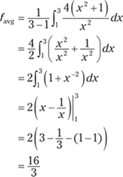
Next, set the original function equal to the average value and solve for c:
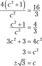
Because ![]() isn't in the specified interval, the solution is
isn't in the specified interval, the solution is ![]() .
.
746. ![]()
Begin by finding the average value of the function on the given interval by using the average value formula with a = 4, b = 9, and ![]() :
:

Next, set the original function equal to the average value and solve for c:

Because ![]() is in the given interval, you've found the solution.
is in the given interval, you've found the solution.
747. ![]()
Begin by finding the average value of the function on the given interval by using the average value formula with a = –2, b = 2, and f (x) = 5 – 3x2:
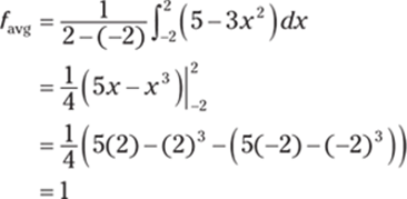
Next, set the original function equal to the average value and solve for c:
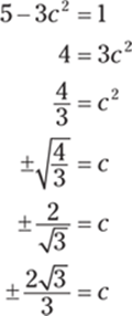
Both values fall in the given interval, so both are solutions.
748. ![]()
Using the average value formula with a = 0, ![]() , and f (x) = x sin x gives you
, and f (x) = x sin x gives you
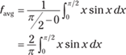
To integrate this function, you can use integration by parts. Notice that for the indefinite integral ![]() , you can let u = x so that du = dx and let dv = sin x dx so that v = –cos x dx. Using integration by parts formula gives you
, you can let u = x so that du = dx and let dv = sin x dx so that v = –cos x dx. Using integration by parts formula gives you

Therefore, to evaluate the definite integral ![]() , you have
, you have
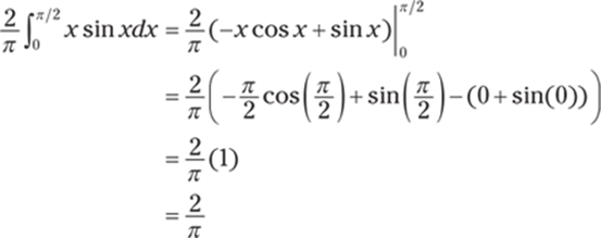
749. 
Using the average value formula with a = 0, ![]() , and
, and ![]() gives you
gives you

To evaluate this integral, begin by splitting up the fraction:

For the first integral, use a substitution, letting u = x2 + 1 so that du = 2x dx, or ![]() . You can also find the new limits of integration for the first integral by noting that if
. You can also find the new limits of integration for the first integral by noting that if ![]() , then
, then  , and if x = 0, then u = 02 + 1 = 1. With these new values, you have
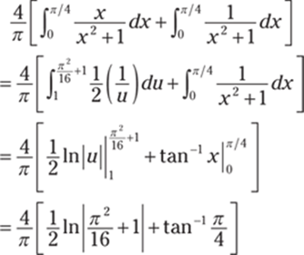
750. 
To find the derivative of ![]() , use the derivative formula for sin−1 x and the chain rule:
, use the derivative formula for sin−1 x and the chain rule:
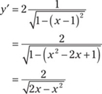
751. 
To find the derivative of ![]() , you need to know the derivative formula for the inverse cosine function and also use the chain rule:
, you need to know the derivative formula for the inverse cosine function and also use the chain rule:
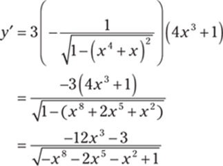
752. 
First rewrite the radical using an exponent:
![]()
Then use the derivative formula for tan−1 x and the chain rule to find the derivative:
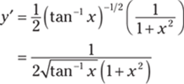
753. 
First rewrite the radical using an exponent:
![]()
Find the derivative using the product rule and the derivative formula for sin−1 x:
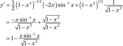
754. ![]()
To find the derivative of ![]() , use the derivative formula for tan−1 x along with the chain rule:
, use the derivative formula for tan−1 x along with the chain rule:

755. 
Find the derivative of ![]() using the chain rule and the derivative formula for sec−1 t:
using the chain rule and the derivative formula for sec−1 t:
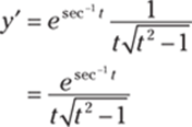
756. 
To find the derivative of y = csc−1 e2x, use the derivative formula for csc−1 x along with the chain rule:
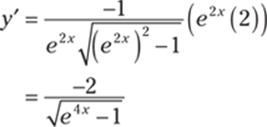
757. 
To find the derivative of ![]() , use the derivative formula for ex along with the chain rule and product rule:
, use the derivative formula for ex along with the chain rule and product rule:
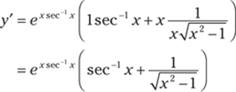
758. 
Rewrite the arccosine as the inverse cosine:
![]()
Now use the chain rule along with the derivative formula for cos−1 x:
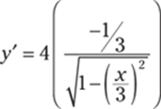
Next, simplify the term underneath the square root. Begin by getting common denominators under the radical:
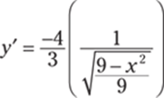
Then split up the square root and simplify:
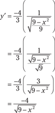
759. ![]()
First, rewrite the radical using an exponent:

Use the product rule on the first term and the chain rule on the second term to get the derivative:

760. 0
Rewrite ![]() in the given function using a negative exponent:
in the given function using a negative exponent:

Use the derivative formula for cot−1 x for the first term, and use the same derivative formula and the chain rule for the second term. Here are the calculations:
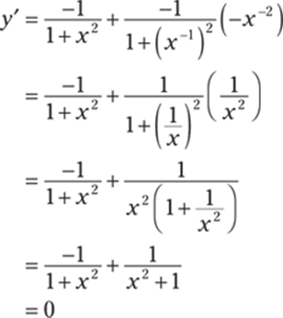
761. 
Here's the given function:
![]()
Begin by using the derivative formula for tan−1 x on the first term and using the quotient rule on the second term:
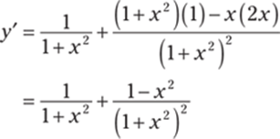
Then get common denominators and simplify:

762. 
Rewrite the radical in the given function using an exponent:

Use the derivative formula for tan−1 x along with the chain rule:

Now the fun algebra simplification begins:
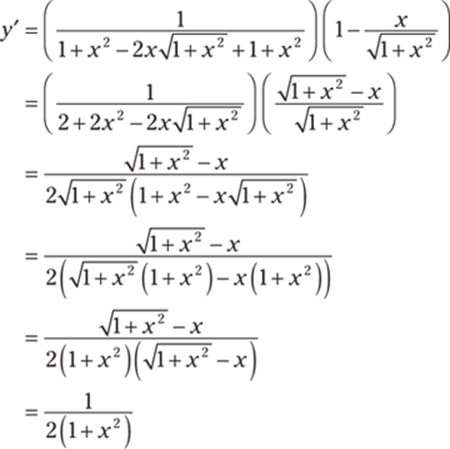
763. ![]()
Here's the initial problem:
![]()
Because you have the antiderivative formula ![]() , you can simply apply that here to find the solution:
, you can simply apply that here to find the solution:
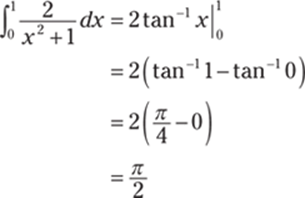
764. ![]()
Here's the given problem:

Because you have the antiderivative formula  , you can simply apply that here to find the solution:
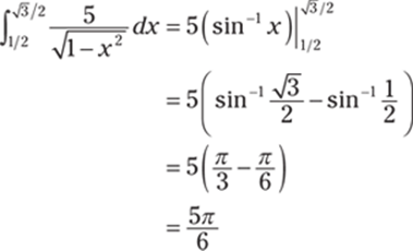
765. ![]()
You may want to write the second term underneath the radical as a quantity squared so you can more easily see which substitution to use:

Now begin by using the substitution u = 3x so that du = 3 dx, or ![]() . This gives you the following:
. This gives you the following:
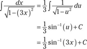
766. ![]()
Here's the given problem:

Begin by using the substitution u = sin−1 x so that  . Find the new limits of integration by noting that if
 ![]() , then
, then ![]() , and if x = 0, then u = sin−1 0 = 0. With these new values, you get the following answer:
, and if x = 0, then u = sin−1 0 = 0. With these new values, you get the following answer:
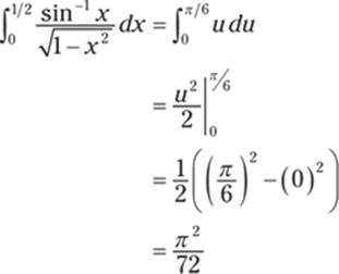
767. ![]()
Here's the given problem:
![]()
Begin with the substitution u = sin x so that du = cos x dx. Notice that if ![]() , then
, then ![]() , and that if x = 0, then u = sin 0 = 0. With these new values, you get the following:
, and that if x = 0, then u = sin 0 = 0. With these new values, you get the following:
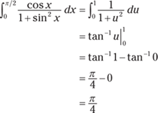
768. ![]()
Start with the given problem:

Use the substitution u = ln x so that ![]() :
:
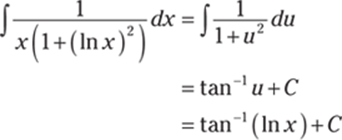
769. ![]()
Here's the given problem:

Begin with the substitution ![]() so that u2 = x and 2u du = dx. Using these substitutions gives you the following:
so that u2 = x and 2u du = dx. Using these substitutions gives you the following:
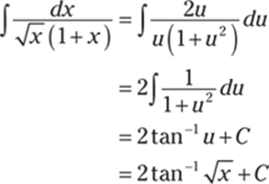
770. ![]()
Here's the given problem:

Begin by doing a bit of algebra to manipulate the denominator of the integrand:
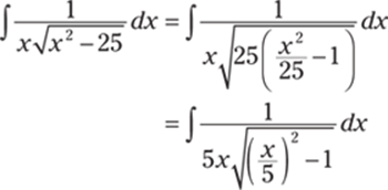
Now use the substitution ![]() so that
so that ![]() , or 5du = dx:
, or 5du = dx:
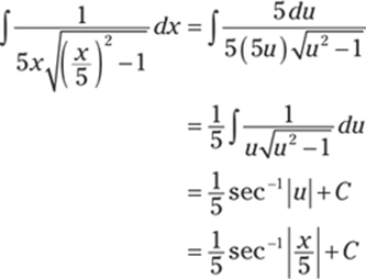
771. ![]()
Here's the given problem:

Begin by completing the square on the expression underneath the square root.

This gives you

Now use the substitution u = x – 1 so that du = dx:
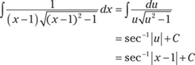
772. ![]()
The given problem is

You'd like to have “1 – (a quantity squared)” under the radical so that you can use the formula  , so you may want to write the second term under theradical as a quantity squared and try a substitution to see whether it all works out. (Of course, you can use the substitution without rewriting, but rewriting may help you see which substitution to use.)

Now you can use the substitution u = e3x so that du = 3e3x dx, or ![]() :
:
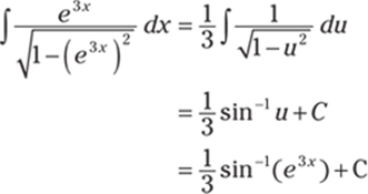
773. ![]()
Begin by splitting the integral:
![]()
For the first integral, you can use the substitution u = x2 + 4 so that du = 2x dx, or ![]() . For the second integral, simply use the tan−1 x formula for integration,which gives you the following:
. For the second integral, simply use the tan−1 x formula for integration,which gives you the following:
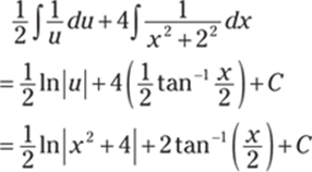
774. ![]()
Here's the given problem:

Begin by completing the square on the expression under the radical:
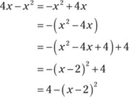
This gives you

Now use the substitution u = x – 2 so that u + 2 = x and du = dx. Notice you can find the new limits of integration by noting that if x = 3, then u = 3 – 2 = 1, and if x = 2, then u = 2 – 2 = 0.

Next, use some algebra to manipulate the expression under the radical:
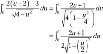
Now you can use the substitution ![]() so that 2w = u and 2 dw = du. You can again find the new upper limit of integration by using the substitution
so that 2w = u and 2 dw = du. You can again find the new upper limit of integration by using the substitution ![]() and noting that when u = 1, you have
and noting that when u = 1, you have ![]() . Likewise, you can find the new lower limit of integration by noting that when u= 0, you have
. Likewise, you can find the new lower limit of integration by noting that when u= 0, you have ![]() .
.
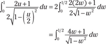
Now split the integral:
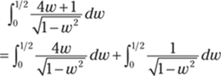
In the first integral, use the substitution v = 1 – w2 so that dv = –2w dw and –2 dv = 4w dw. You can again update the limits of integration by using the substitution v = 1 – w2. To find the new upper limit of integration, note that when ![]() , you have
, you have  . To find the new lower limit of integration, note that when w = 0, you have v = 1 – 02 = 1. Again, use this substitution only for the first integral:
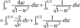
Reverse the bounds in the first integral and change the sign. Then simplify:
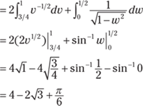
Whew!
775. 0
Using the definition of hyperbolic sine gives you the following:
![]()
776. ![]()
Using the definition of hyperbolic cosine gives you the following:
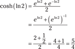
777. ![]()
Using the definition of hyperbolic cotangent gives you the following:
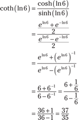
778. ![]()
Using the definition of hyperbolic tangent gives you the following:
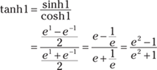
779. ![]()
Using the definition of hyperbolic cosine gives you the following:
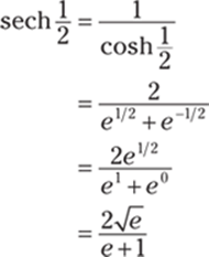
780. 2 cosh x sinh x
The given function is y = cosh2 x, which equals (cosh x)2. Using the chain rule gives you the derivative y′ = 2 cosh x sinh x.
781. ![]()
The given function is ![]() . Using the chain rule gives you
. Using the chain rule gives you

782. ![]()
Here's the given function:
![]()
Use the chain rule to find the derivative:

783. ![]()
Here's the given function:
![]()
Use the chain rule to find the derivative:

784. ![]()
The given function is
y = tanh(sinh x)
Use the chain rule to get the derivative:

785. ![]()
Here's the given function:
![]()
Use the chain rule to find the derivative:

786. ![]()
Rewrite the given function:
![]()
Then use the chain rule to find the derivative:

787. 
Here's the given function:
![]()
Use the chain rule to find the derivative:

788. 2x3 – x
Before taking the derivative, simplify the function:
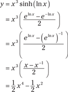
Now simply take the derivative using the power rule:

789. ![]()
The given function is

Use the chain rule to find the derivative:

Rewrite and simplify the equation to get the answer:

790. ![]()
Here's the given problem:
![]()
To find the antiderivative, use the substitution u = 1 – 3x so that du = –3 dx, or ![]() :
:
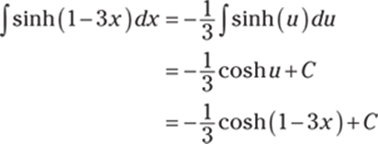
791. ![]()
Here's the given problem:
![]()
To find the antiderivative, begin by using the substitution u = cosh (x – 3) so that du = sinh (x – 3) dx. With this substitution, you get the following:
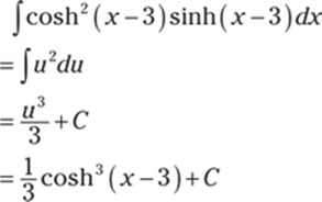
792. ![]()
Rewrite the problem using the definition of hyperbolic cotangent:
![]()
Begin finding the antiderivative by using the substitution u = sinh x so that du = cosh x dx. With these substitutions, you get the following:
![]()
793. ![]()
Here's the given problem:
![]()
To find the antiderivative, use the substitution u = 3x – 2 to get du = 3 dx so that ![]() . With these substitutions, you get the following:
. With these substitutions, you get the following:

794. ![]()
The given problem is
![]()
Begin by using the substitution u = 2 + tanh x so that du = sech2 x dx:

795. ![]()
Here's the given problem:
![]()
To find the antiderivative, use integration by parts with u = x so that du = dx, and let dv = cosh(6x) dx so that ![]() . This gives you the following:
. This gives you the following:
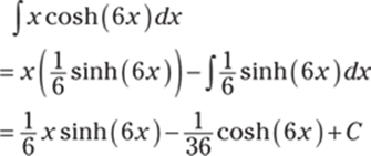
796. 
Here's the given problem:

To find the antiderivative, begin by using the substitution ![]() so that
so that ![]() , or
, or ![]() . With these substitutions, you get the following:
. With these substitutions, you get the following:

797. 
Start with the given problem:

To find the antiderivative, begin by using the substitution ![]() so that du = –2x−3,or
so that du = –2x−3,or ![]() . With these substitutions, you get the following:
. With these substitutions, you get the following:
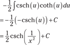
798. ![]()
The given problem is
![]()
To find the antiderivative, begin by using the hyperbolic identity cosh2 x – 1 = sinh2 x:
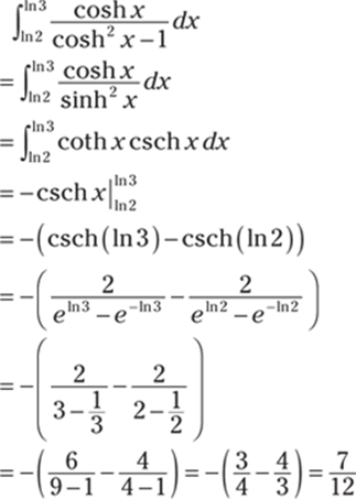
799. ![]()
Here's the given problem:

To find the antiderivative, begin by using the substitution u = sinh x so that du = cosh x dx. You can find the new limits of integration by noting that if x = ln 2, then  , and if x = 0, then
 ![]() . With these substitutions, you produce the following:
. With these substitutions, you produce the following:
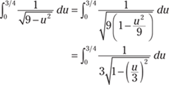
Now use a new substitution ![]() so that
so that ![]() , or 3 dw = du. You can again find the new limits of integration by noting that if
, or 3 dw = du. You can again find the new limits of integration by noting that if ![]() , then
, then  , and if u = 0, then
 ![]() . With these substitutions, you get the following:
. With these substitutions, you get the following:
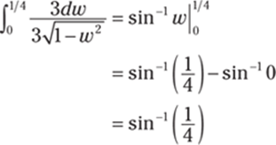
800. 3
The given problem is
![]()
Notice that if you substitute in the value x = –1, you get the indeterminate form ![]() . Now use L'Hôpital's rule to find the limit:
. Now use L'Hôpital's rule to find the limit:
![]()
801. ![]()
Here's the given problem:
![]()
Notice that if you substitute in the value x = 1, you get the indeterminate form ![]() . Using L'Hôpital's rule gives you the limit:
. Using L'Hôpital's rule gives you the limit:

802. ![]()
Start with the given problem:
![]()
Notice that if you substitute in the value x = 2, you get the indeterminate form ![]() . Use L'Hôpital's rule to find the limit:
. Use L'Hôpital's rule to find the limit:

803. ∞
The given problem is

Notice that if you substitute in the value ![]() , you get the indeterminate form
, you get the indeterminate form ![]() . Using L'Hôpital's rule gives you the limit:
. Using L'Hôpital's rule gives you the limit:

804. 0
Start with the given problem:
![]()
Notice that if you substitute in the value x = 0, you get the indeterminate form ![]() . Use L'Hôpital's rule to find the limit:
. Use L'Hôpital's rule to find the limit:
![]()
805. 0
Here's the given problem:
![]()
Notice that if you take the limit, you get the indeterminate form ![]() . Using L'Hôpital's rule gives you the limit as follows:
. Using L'Hôpital's rule gives you the limit as follows:

806. ![]()
Here's the given problem:

Notice that if you substitute in the value x = 1, you get the indeterminate form ![]() . Using L'Hôpital's rule gives you
. Using L'Hôpital's rule gives you

807. 1
The given problem is
![]()
Notice that if you substitute in the value x = 0, you get the indeterminate form ![]() . Using L'Hôpital's rule gives you the limit:
. Using L'Hôpital's rule gives you the limit:

808. ![]()
Here's the given problem:

Applying the limit gives you the indeterminate form ∞ – ∞. Write the expression as a single fraction by getting common denominators and then apply L'Hôpital's rule:
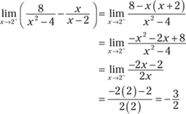
809. ![]()
The given problem is

Notice that if you substitute in the value x = 0, you get the indeterminate form ![]() . Apply L'Hôpital's rule to find the limit:
. Apply L'Hôpital's rule to find the limit:
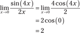
810. 0
Here's the given problem:
![]()
Applying the limit gives you the indeterminate form 0(–∞). Rewrite the product as a quotient and use L'Hôpital's rule to find the limit:
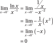
811. 0
Here's the given problem:
![]()
Applying the limit gives you the indeterminate form ![]() . Use properties of logarithms to rewrite the expression and then use L'Hôpital's rule to find the limit:
. Use properties of logarithms to rewrite the expression and then use L'Hôpital's rule to find the limit:

812. 1
The given problem is
![]()
Substituting the value x = 0 gives you the indeterminate form ![]() . Apply L'Hôpital's rule to find the limit:
. Apply L'Hôpital's rule to find the limit:

813. 0
Here's the initial problem:

Make sure you have an indeterminate form before applying L'Hospital's rule, or you can get incorrect results! Notice that as x → ∞ in the numerator, ![]() →
→ ![]() , and as x → ∞ in the denominator, (x – 1) → ∞. Therefore, the solution becomes
, and as x → ∞ in the denominator, (x – 1) → ∞. Therefore, the solution becomes

814. –∞
Here's the given problem:

Applying the limit gives you the indeterminate form ![]() . Applying L'Hôpital's rule gives you the following:
. Applying L'Hôpital's rule gives you the following:
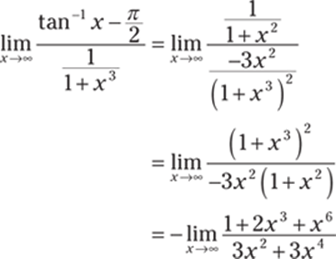
This limit is still an indeterminate form, and you can continue using L'Hôpital's rule four more times to arrive at the solution. However, because the degree of the numerator is larger than the degree of the denominator, you can find the limit by noting that
![]()
815. 0
The given problem is
![]()
Applying the limit gives you the indeterminate form ∞ – ∞. Rewrite the difference as a quotient and use L'Hôpital's rule:
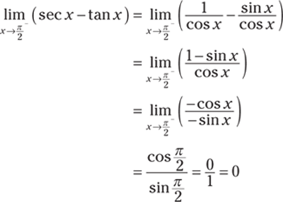
816. ![]()
Start with the given problem:
![]()
Applying the limit gives you the indeterminate form (∞)(0). Rewrite the product as a quotient and use L'Hôpital's rule as follows:
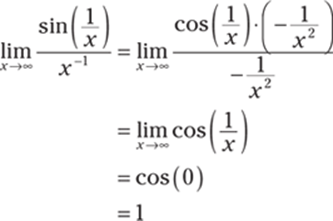
817. 0
Here's the initial problem:
![]()
Taking the limit gives you the indeterminate form (–∞)(0). Rewrite the product as a quotient and use L'Hôpital's rule:
![]()
Applying the limit again gives you the indeterminate form ![]() . Using L'Hôpital's rule again gives you the following:
. Using L'Hôpital's rule again gives you the following:
![]()
If you again take the limit, you get the indeterminate form ![]() . Use L'Hôpital's rule one more time to get the final answer:
. Use L'Hôpital's rule one more time to get the final answer:
![]()
818. 1
The given problem is
![]()
Applying the limit gives you the indeterminate form ∞ – ∞. Begin by factoring out x; then rewrite the expression as a fraction and use L'Hôpital's rule:
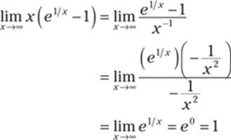
819. ∞
The given problem is
![]()
Substituting in the value x = ∞ gives you the indeterminate form ![]() , so use L'Hôpital's rule:
, so use L'Hôpital's rule:

If you again substitute in the value x = ∞, you still get the indeterminate form ![]() . Applying L'Hôpital's rule one more time gives you the limit:
. Applying L'Hôpital's rule one more time gives you the limit:

820. ![]()
Here's the initial problem:
![]()
Substituting in the value x = 1 gives you the indeterminate form ![]() , so use L'Hôpital's rule:
, so use L'Hôpital's rule:

If you again substitute in the value x = 1, you still get the indeterminate form ![]() . Using L'Hôpital's rule again gives you the limit:
. Using L'Hôpital's rule again gives you the limit:
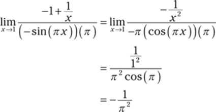
821. e−5
Here's the given problem:
![]()
Substituting in the value x = 0 gives you the indeterminate form 1∞. Create a new limit by taking the natural logarithm of the original expression, ![]() , so that
, so that ![]() , or
, or  . Take the limit of the new expression:

Then apply L'Hôpital's rule:
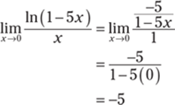
Because ![]() and
and ![]() , it follows that
, it follows that
![]()
822. 1
Here's the initial problem:
![]()
Applying the limit gives you the indeterminate form ∞0. Create a new limit by taking the natural logarithm of the original expression, ![]() , so that
, so that ![]() , or
, or ![]() . Then take the limit of this new expression:
. Then take the limit of this new expression:
![]()
Apply L'Hôpital's rule:

Because ![]() and
and ![]() , it follows that
, it follows that
![]()
823. 1
Here's the given problem:
![]()
Applying the limit gives you the indeterminate form 1∞. Create a new limit by taking the natural logarithm of the original expression, y = (cos x)2/x, so that ln y = ln(cos x)2/x, or  . Then take the limit of this new expression:

Apply L'Hôpital's rule:
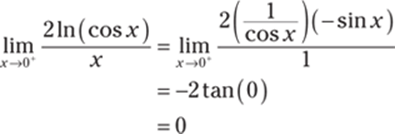
Because ![]() and
and ![]() , it follows that
, it follows that
![]()
824. e−15/9
The given problem is

Applying the limit gives you the indeterminate form 1∞. Create a new limit by taking the natural logarithm of the original expression,  , so that
  , or
, or ![]() . Next, rewrite the expression as a fraction and use properties of logarithms to expand the natural logarithm (this step will make finding the derivative a bit easier):
. Next, rewrite the expression as a fraction and use properties of logarithms to expand the natural logarithm (this step will make finding the derivative a bit easier):

Apply L'Hôpital's rule:
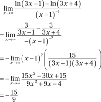
Because  and
and ![]() , it follows that
, it follows that

825. 1
Here's the given problem:
![]()
Substituting in the value x = 0 gives you the indeterminate form 00. Create a new limit by taking the natural logarithm of the original expression, ![]() , so that
, so that ![]() , or
, or ![]() . Then take the limit of the new expression:
. Then take the limit of the new expression:

Apply L'Hôpital's rule:

Because ![]() and
and ![]() , it follows that
, it follows that
![]()
826. 1
Here's the given problem:
![]()
Substituting in the value x = 0 gives you the indeterminate form 00. Create a new limit by taking the natural logarithm of the original expression, ![]() , so that
, so that ![]() , or
, or ![]() . Next, take the limit of the new expression:
. Next, take the limit of the new expression:
![]()
Apply L'Hôpital's rule:

Rewrite the expression and simplify:
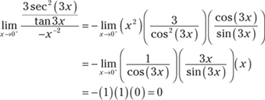
Because ![]() and
and ![]() , it follows that
, it follows that
![]()
827. 0
The given problem is
![]()
Applying the limit gives you the indeterminate form 0(–∞). Rewrite the product as a quotient and use L'Hôpital's rule to get the limit:
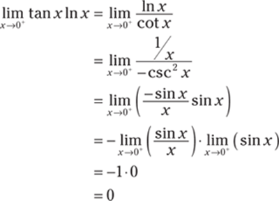
828. e
Here's the initial problem:
![]()
Applying the limit gives you the indeterminate form 1∞. Create a new limit by taking the natural logarithm of the original expression, ![]() , so that
, so that ![]() , or
, or ![]() . Noting that
. Noting that ![]() is an indeterminate product, you can rewrite this limit as
is an indeterminate product, you can rewrite this limit as

Next, apply L'Hôpital's rule:
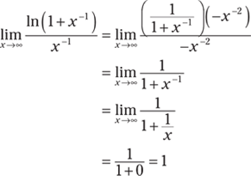
Because ![]() and
and ![]() , it follows that
, it follows that
![]()
829. e4
The given problem is
![]()
Applying the limit gives you the indeterminate form 1∞. Create a new limit by taking the natural logarithm of the original expression, ![]() , so that
, so that ![]() , or
, or  . Then use L'Hôpital's rule on the new limit:
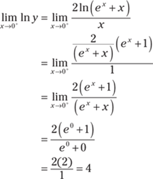
Because ![]() and
and ![]() , it follows that
, it follows that
![]()
830. –∞
Here's the given problem:

Applying the limit gives you the indeterminate form ∞ – ∞, so write the expression as a single fraction by getting common denominators and then apply L'Hôpital's rule:

Multiply the numerator and denominator by x:

Notice that as x → 1+ in the numerator, 2x2 (ln x) – x2 → –1, and as x → 1+ in the denominator, x2 – 1 + 2x2 ln x → 0+. Therefore, you get the following answer:
![]()
831. ![]()
Here's the given problem:
![]()
Evaluating the limit gives you the indeterminate form ∞ – ∞, so write the expression as a single fraction by getting a common denominator and then use L'Hôpital's rule:

Multiply the numerator and denominator by x:
![]()
Substituting in the value x = 1 gives you the indeterminate form ![]() , so you can again use L'Hôpital's rule:
, so you can again use L'Hôpital's rule:
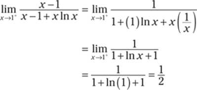
832. ![]()
Here's the given integral:
![]()
If you let u = 5x, then du = 5dx, or ![]() . Substituting into the original integral, you get
. Substituting into the original integral, you get
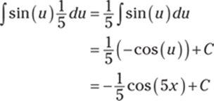
833. ![]()
Here's the given integral:
![]()
If you let u = x + 4, then du = dx. Substituting into the original integral gives you the following:

834. ![]()
The given integral is
![]()
If you let u = x3 + 1, then du = 3x2 dx. Substitute into the original integral and solve:
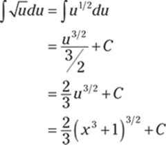
835. ![]()
The given integral is

If you let ![]() , then you get
, then you get ![]() , or equivalently,
, or equivalently, ![]() . Substitute into the original integral:
. Substitute into the original integral:

836. ![]()
Here's the given integral:

If you let u = 4 + 5x, then you get du = 5 dx, or ![]() . Substitute into the original integral:
. Substitute into the original integral:
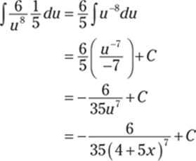
837. ![]()
Start by rewriting the given integral:
![]()
If you let ![]() , then
, then ![]() . Substitute into the original integral to find the answer:
. Substitute into the original integral to find the answer:
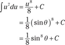
838. 0
Recall that ![]() is an odd function; that is,
is an odd function; that is, ![]() . Likewise,
. Likewise, ![]() so that
so that ![]() is also an odd function. Because this function is symmetric about the origin and you're integrating over an interval of the form [–a, a], you get
is also an odd function. Because this function is symmetric about the origin and you're integrating over an interval of the form [–a, a], you get ![]() .
.
Here's an alternate approach: Begin by saving a factor of the tangent and use an identity to allow you to split up the integral:
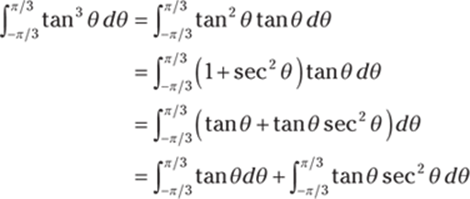
To evaluate the first integral, rewrite the tangent:
![]()
Then use the substitution ![]() so that
so that ![]() , or
, or ![]() . You can find the new limits of integration by noting that if
. You can find the new limits of integration by noting that if ![]() or if
or if ![]() , you have
, you have ![]() :
:
![]()
Because the upper and lower limits of integration are the same, you have the following for the first integral:
![]()
The second integral is
![]()
To evaluate the second integral, use the substitution ![]() so that
so that ![]() . Notice that you can find the new limits of integration by noting that if
. Notice that you can find the new limits of integration by noting that if ![]() , then
, then ![]() , and if
, and if ![]() , then
, then ![]() . Therefore, the second integral becomes
. Therefore, the second integral becomes
![]()
Combining the values of the first and second integrals gives you the answer:
![]()
839. 4
The given integral is
![]()
Start by using the substitution u = ln x so that ![]() . You can find the new limits of integration by noting that if x = e2, then u = ln e2 = 2, and if x = 1, then u = ln 1 = 0. Therefore, the integral becomes
. You can find the new limits of integration by noting that if x = e2, then u = ln e2 = 2, and if x = 1, then u = ln 1 = 0. Therefore, the integral becomes
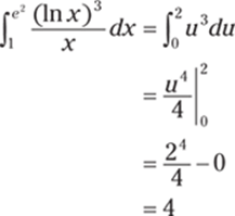
840. ![]()
The given integral is
![]()
Start by letting u = 4 – 3x so that du = –3dx, or ![]() . Substitute this back into the original integral:
. Substitute this back into the original integral:

841. ![]()
Here's the given integral:
![]()
Let u = tan−1 x so that ![]() . Substituting these values into the original integral, you get
. Substituting these values into the original integral, you get

842. ![]()
Start by rewriting the integral:
![]()
Now you can perform a u-substitution with u = cos x so that du = –sin x dx, or –du = sin x dx. Substituting this expression into the original integral gives you the following:

You can now use the power property of logarithms to rewrite the integral:
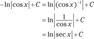
![]()
843. e – e1/2
The given integral is
![]()
Begin by using the substitution u = cos x so that du = –sin x dx, or –du = sin x dx. Notice you can find the new limits of integration by noting that if ![]() , then
, then ![]() , and if x = 0, then u = cos 0 = 1. With these values, you have the following:
, and if x = 0, then u = cos 0 = 1. With these values, you have the following:
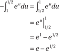
844. ![]()
Rewrite the given integral:
![]()
Begin by using the substitution u = 1 + x3/2 so that ![]() , or
, or ![]() . Notice you can find the new limits of integration by noting that if x = 1, then u = 1 + 13/2 = 2, and if x = 0, then u = 1 + 03/2 = 1. With these new values, you find that
. Notice you can find the new limits of integration by noting that if x = 1, then u = 1 + 13/2 = 2, and if x = 0, then u = 1 + 03/2 = 1. With these new values, you find that

845. ![]()
Rewrite the given integral:
![]()
Then use the substitution u = tan x so that du = sec2 x dx:
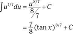
846. ![]()
Here's the given integral:

Use the substitution ![]() so that
so that ![]() , or
, or ![]() :
:
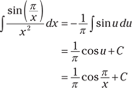
847. ![]()
Here's the given integral:

If you let u = 1 + 2x + 3x2, then you get du = (2 + 6x)dx, or 2du = (4 + 12x)dx. Substitute this value into the original integral:
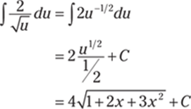
848. ![]()
Here's the given integral:
![]()
If you let u = cot x, then you get du = –csc2 x dx, or –du = csc2 x dx. Substitute this value into the original integral:
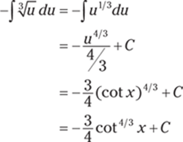
849. ![]()
Here's the given integral:
![]()
If you let u = x2, then du = 2x dx, or ![]() . You can also find the new limits of integration by using the original limits of integration along with the u-substitution. When
. You can also find the new limits of integration by using the original limits of integration along with the u-substitution. When ![]() ,
,  . Likewise, if x = 0, then u = (0)2 = 0.
Now substitute these values into the original integral:
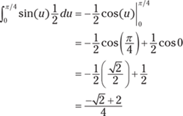
850. ![]()
The given integral is
![]()
Begin by breaking the integral into two separate integrals:

Notice that  .
.
All that's left is to integrate the second integral; you can do this with a u-substitution. For  , let u = 1 + x2 so that du = 2x dx, or
 ![]() . Substituting these values into the second integral gives you the following:
. Substituting these values into the second integral gives you the following:

The expression 1 + x2 is always positive, so you can drop the absolute value sign:
![]()
Combining the solutions gives you
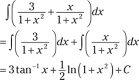
851. ![]()
The given integral is

Begin with the u-substitution u = ln x so that ![]() . You can also compute the new limits of integration by noting that if x = e, then u = ln e = 1, and if x = e2, then u = ln e2 = 2. Now you can integrate:
. You can also compute the new limits of integration by noting that if x = e, then u = ln e = 1, and if x = e2, then u = ln e2 = 2. Now you can integrate:
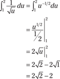
852. ![]()
Here's the given integral:
![]()
Start with the substitution ![]() so that
so that ![]() . Substituting these values into the original integral, you get the following:
. Substituting these values into the original integral, you get the following:

853. ![]()
The given integral is
![]()
Begin by letting u = –x3 so that du = –3x2 dx, or ![]() . Substitute these values into the original integral:
. Substitute these values into the original integral:

854. ![]()
Here's the given integral:
![]()
Begin by using the substitution u = x + 1 so that u – 1 = x and du = dx. Notice you can find the new limits of integration by noting that if x = 3, then u = 3 + 1 = 4, and if x = 0, then u = 0 + 1 = 1. With these new values, you have the following:
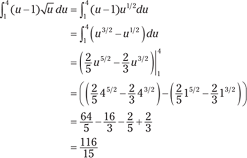
855. 
At first, you may have trouble seeing how a substitution will work for this problem. But note that you can split x5 into x3x2:
![]()
Now you can use the substitution u = x3 + 1 so that u – 1 = x3 and du = 3x2 dx, or ![]() . Notice that you can find the new limits of integration by noting that if x = 1, then u = 13 + 1 = 2, and if x = 0, then u = 03 + 1 = 1. With these values, you get the following integral:
. Notice that you can find the new limits of integration by noting that if x = 1, then u = 13 + 1 = 2, and if x = 0, then u = 03 + 1 = 1. With these values, you get the following integral:
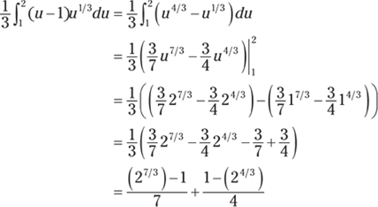
856. ![]()
Here's the given integral:
![]()
If you let u = x + 3, then du = dx and u – 3 = x. Substituting into the original integral, you get the following:
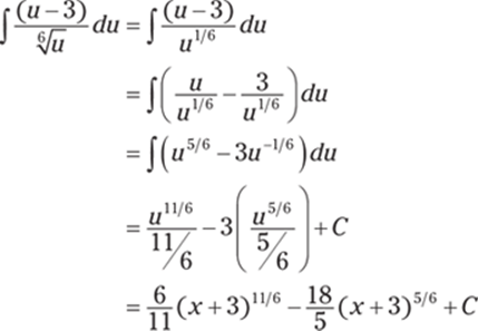
857. ![]()
At first glance, substitution may not seem to work for this problem. However, you can rewrite the integral as follows:
![]()
If you let u = x4 + 1, then you get du = 4x3 dx, or ![]() . Notice also from the u-substitution that u – 1 = x4. Substitute into the original integral and simplify:
. Notice also from the u-substitution that u – 1 = x4. Substitute into the original integral and simplify:
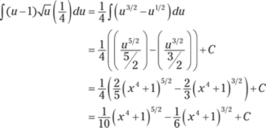
858. ![]()
The given integral is
![]()
Use integration by parts with u = x so that du = dx and let dv = cos(4x) dx so that ![]() . Using the integration by parts formula gives you the following:
. Using the integration by parts formula gives you the following:
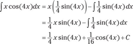
859. ![]()
Here's the given integral:
![]()
Use integration by parts with u = x so that du = dx and let dv = ex dx so that v = ex. Using the integration by parts formula gives you the following:

860. ![]()
Here's the given integral:
![]()
Use integration by parts with u = x so that du = dx and let dv = sinh(2x) dx so that ![]() . Using the integration by parts formula gives you the following:
. Using the integration by parts formula gives you the following:

861. 
The given integral is
![]()
Use integration by parts with u = x so that du = dx and let dv = 6x dx so that ![]() . Using the integration by parts formula gives you the following:
. Using the integration by parts formula gives you the following:
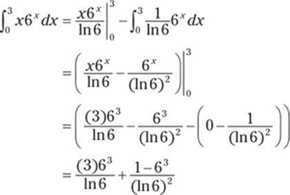
862. ![]()
The given integral is
![]()
Use integration by parts with u = x so that du = dx and let dv = sec x tan xdx so that v = sec x:

863. ![]()
The given integral is
![]()
Begin by using integration by parts with u = x so that du = dx and let dv = sin(5x) dx so that ![]() :
:

864. ![]()
The given integral is
![]()
Begin by using integration by parts with u = x so that du = dx and let dv = csc2 x dx so that v = –cot x:

865. –x cos x + sin x + C
The given integral is
![]()
Use integration by parts with u = x so that du = dx and let dv = sin x dx so that v = –cos x:

866. ![]()
Here's the given integral:
![]()
Use integration by parts with u = x so that du = dx and let dv = csc x cot x dx so that v = –csc x:

867. ![]()
The given integral is
![]()
Use integration by parts with u = ln(3x + 1) so that ![]() and let dv = dx so that v = x. Using the integration by parts formula gives you
and let dv = dx so that v = x. Using the integration by parts formula gives you
![]()
To evaluate the integral ![]() , you can use long division to simplify, or you can add 1 and subtract 1 from the numerator and split up the fraction:
, you can use long division to simplify, or you can add 1 and subtract 1 from the numerator and split up the fraction:
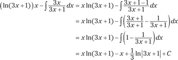
868. ![]()
The given integral is
![]()
Use integration by parts with u = tan−1 x so that ![]() and let dv = dx so that v = x. Using the integration by parts formula gives you
and let dv = dx so that v = x. Using the integration by parts formula gives you
![]()
To evaluate ![]() , use the substitution u1 = 1 + x2 so that du1 = 2x dx, or
, use the substitution u1 = 1 + x2 so that du1 = 2x dx, or ![]() . With these substitutions, you get the following:
. With these substitutions, you get the following:

869. ![]()
The given integral is
![]()
Use integration by parts with u = ln x so that ![]() and let dv = x−2 dx so that
and let dv = x−2 dx so that ![]() . Using the integration by parts formula gives you the following:
. Using the integration by parts formula gives you the following:
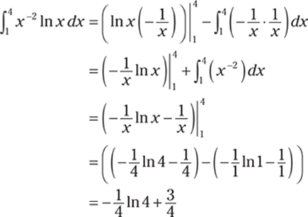
870. 4e3
Here's the given integral:
![]()
Begin by using the substitution ![]() so that w2 = x and 2w dw = dx. You can find the new limits of integration by noting that if x = 9, then
so that w2 = x and 2w dw = dx. You can find the new limits of integration by noting that if x = 9, then ![]() , and if x = 1, then
, and if x = 1, then ![]() . These substitutions give you the following:
. These substitutions give you the following:
![]()
Use integration by parts with u = 2w so that du = 2dw and let dv = ew dw so that v = ew. Using the integration by parts formula gives you the following:
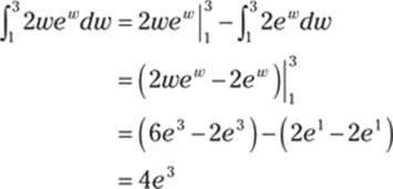
871. ![]()
The given integral is
![]()
Use integration by parts with u = ln x so that ![]() and let dv = x3/2 dx so that
and let dv = x3/2 dx so that ![]() to get the following:
to get the following:
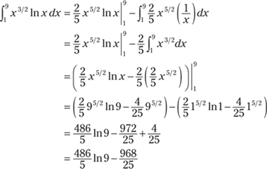
872. ![]()
Here's the given integral:
![]()
Use integration by parts with u = cos−1 x so that  and let dv = 1dx so that v = x:
![]()
Next, use the substitution w = 1 – x2 so that dw = –2x dx, or ![]() :
:
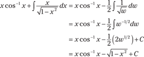
873. ![]()
The given integral is
![]()
Use integration by parts with u = sin−1(5x) so that  and let dv = 1dx so that v = x:

Next, use the substitution w = 1 – 25x2 so that dw = –50x dx, or ![]() :
:
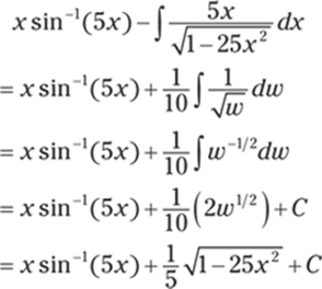
874. ![]()
Here's the given integral:
![]()
Begin by using integration by parts with u = x2 so that du = 2x dx and let dv = e−2x so that ![]() :
:

Use integration by parts again with u1 = x so that du1 = dx and let dv1 = e−2x so that ![]() :
:
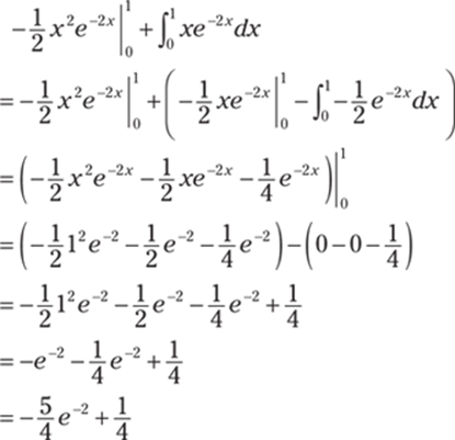
875. –6e−1 + 3
The given integral is
![]()
Begin by using integration by parts with u = x2 + 1 so that du = 2x dx and let dv = e–x dx so that v = –e–x:
![]()
Now use integration by parts again with u1 = 2x so that du1 = 2 dx and let dv1 = e–x dx so that v1 = –e–x:
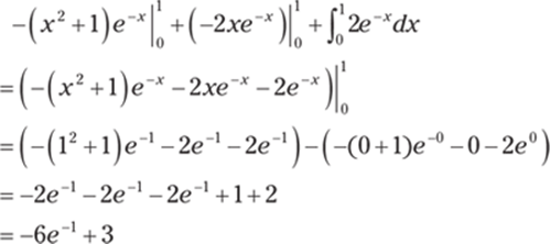
876. ![]()
Here's the given integral:
![]()
Begin by using the substitution w = x2 so that dw = 2x dx, or ![]() , to get the following:
, to get the following:
![]()
Next, use integration by parts with u = w so that du = dw and let dv = cos w dw so that v = sin w:
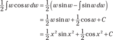
877. ![]()
The given integral is
![]()
Use integration by parts with u = x2 so that du = 2x dx and let dv = sin(mx) dx so that ![]() . Using the integration by parts formula gives you the following:
. Using the integration by parts formula gives you the following:

To evaluate ![]() , use integration by parts again with u1 = x so that du1 = dx and let dv1 = cos(mx) so that
, use integration by parts again with u1 = x so that du1 = dx and let dv1 = cos(mx) so that ![]() . This gives you the following:
. This gives you the following:

Therefore,

878. ![]()
Here's the given integral:
![]()
Begin by using integration by parts with u = (ln x)2 so that ![]() and let dv = x5 dx so that
and let dv = x5 dx so that ![]() . This gives you the following:
. This gives you the following:

To evaluate the new integral, use integration by parts with u1 = ln x so that ![]() and let dv1 = x5 dx so that
and let dv1 = x5 dx so that ![]() . This gives you the following:
. This gives you the following:
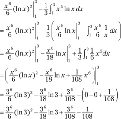
879. ![]()
The given integral is
![]()
Begin by using integration by parts with u = cos(2x) so that du = –2sin(2x)dx and let dv = ex dx so that v = ex. Using the integration by parts formula gives you the following:
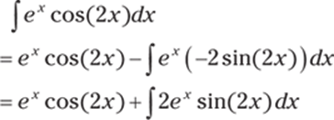
Use integration by parts again with u1 = sin(2x) so that du1 = 2 cos(2x) and let dv1 = ex dx so that v1 = ex. Now you have the following:

Set the expression equal to the original integral:
![]()
Add ![]() to both sides of the equation (note the addition of C1 on the right):
to both sides of the equation (note the addition of C1 on the right):
![]()
Dividing both sides of the equation by 3 yields the solution:
![]()
Note: Don't be thrown off by the constant of integration that switches from C1 to C; they're both arbitrary constants, but simply using ![]() in both equations would be poor notation.
in both equations would be poor notation.
880. –cos x ln(cos x) + cos x + C
Here's the given integral:
![]()
Begin by using the substitution w = cos x so that dw = –sin xdx, or –dw = sin x dx. Using these substitutions gives you the following:
![]()
Now use integration by parts with u = ln w so that ![]() and let dv = –1 dw so that v = –w. Using the integration by parts formula now gives you
and let dv = –1 dw so that v = –w. Using the integration by parts formula now gives you
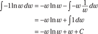
Replacing w with the original substitution, cos x, gives you the solution:
![]()
![]()
881. ![]()
The given integral is
![]()
Begin by using the substitution ![]() so that w2 = x and 2wdw = dx. This gives you the following:
so that w2 = x and 2wdw = dx. This gives you the following:
![]()
Now use integration by parts with u = 2w so that du = 2dw and let dv = cos w dw so that v = sin w:

Using the original substitution, ![]() , gives you the solution:
, gives you the solution:

882. ![]()
Here's the given integral:
![]()
Begin by using integration by parts with u = (ln x)2 so that ![]() and let dv = x4 dx so that
and let dv = x4 dx so that ![]() :
:

To evaluate the new integral, use integration by parts again with u1 = ln x so that ![]() and let dv = x4 dx so that
and let dv = x4 dx so that ![]() :
:
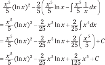
883. ![]()
Here's the given integral:
![]()
Use integration by parts with u = tan−1 x so that ![]() and let dv = x dx so that
and let dv = x dx so that ![]() :
:
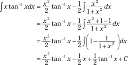
Note: The numerator and denominator are almost the same for the expression ![]() , allowing you to add 1 and subtract 1 (in the second line) and then break it up into two fractions (in the third line); this approach lets you avoid long division. Another way to simplify
, allowing you to add 1 and subtract 1 (in the second line) and then break it up into two fractions (in the third line); this approach lets you avoid long division. Another way to simplify ![]() is to use polynomial long division to arrive at
is to use polynomial long division to arrive at ![]() .
.
884. ![]()
Here's the given integral:
![]()
Recall that ![]() so that
so that ![]() . Using this identity in the integral gives you
. Using this identity in the integral gives you
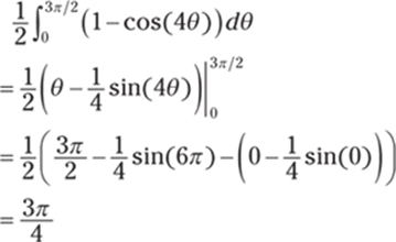
885. ![]()
The given integral is
![]()
Recall that ![]() . Using this identity gives you the following:
. Using this identity gives you the following:
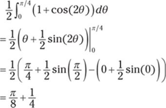
886. ![]()
Here's the given integral:
![]()
As long as you remember your fundamental trigonometric identities, this problem is an easy one!

887. ![]()
The given integral is
![]()
Begin by factoring out sec2 t and using a trigonometric identity on one sec2 t to write it in terms of tan t:

Now use the substitution u = tan t so that du = sec2 t dt. Using these values in the integral gives you
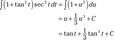
888. ![]()
The given integral is
![]()
Begin by applying the identity ![]() to the integrand to produce the following integral:
to the integrand to produce the following integral:
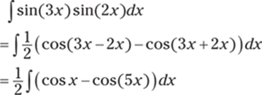
The first term has an elementary antiderivative. To integrate the second term, you can use the substitution u = 5x:
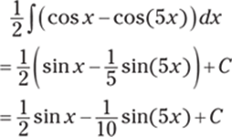
889. ![]()
The given integral is
![]()
Begin by using the identity ![]() on the integrand to produce the following integral:
on the integrand to produce the following integral:
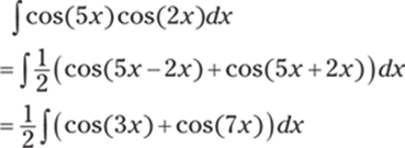
To integrate, use the substitution u = 3x on the first term and the substitution u = 7x on the second term:
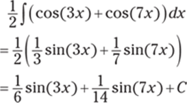
890. ![]()
The given integral is
![]()
Use the substitution u = sin x so that du = cos x dx:
![]()
891. ![]()
The given integral is
![]()
Begin by using the substitution u = tan x so that du = sec2 x dx:
![]()
892. ![]()
Here's the given integral:
![]()
Begin by applying the identity ![]() to the integrand to produce the integral
to the integrand to produce the integral ![]() . Now simplify and integrate:
. Now simplify and integrate:
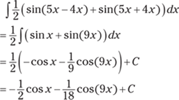
893. sec x + C
Here's the given integral:
![]()
There's a simple solution for this function:
![]()
894. ![]()
Start by rewriting the radical:

Use the substitution u = csc x so that du = –csc x cot x dx, or –du = csc x cot x dx:
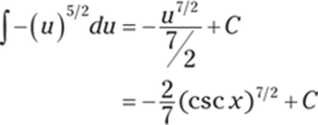
895. ![]()
Here's the given integral:
![]()
Begin by factoring out cos x and using a trigonometric identity to write cos2 x in terms of sin x:

Now use the substitution u = sin x, which gives you du = cos x dx. Putting these values into the integral gives you the following:
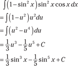
896. ![]()
The given integral is
![]()
Begin by factoring out sec2 x and using a trigonometric identity on one factor of sec2 x to write it in terms of tan x:
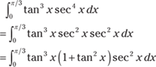
Now use the substitution u = tan x so that du = sec2 x dx. You can also change the limits of integration by noting that if ![]() , then
, then ![]() , and if x = 0, then u = tan 0 = 0. With these new values, the integral becomes
, and if x = 0, then u = tan 0 = 0. With these new values, the integral becomes
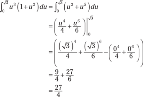
897. ![]()
The given integral is
![]()
Begin by rewriting the integral and factoring out csc2 x:

Now use an identity to get the following:
![]()
Next, use the substitution u = cot x to get du = –csc2 x dx so that

898. ![]()
Here's the given integral:
![]()
Begin by factoring out cos x and using a trigonometric identity to write cos2 x in terms of sin x:
![]()
Now use the substitution u = sin x, which gives you du = cos x dx. You can also find the new limits of integration. If ![]() , then
, then ![]() , and if x = 0, then u = sin 0 = 0. Using these values in the integral gives you
, and if x = 0, then u = sin 0 = 0. Using these values in the integral gives you
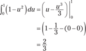
899. ![]()
The given integral is
![]()
Start by rewriting the integrand as two terms:
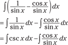
Recall that ![]() . To evaluate
. To evaluate ![]() , use the substitution u = sin x so that du = cos x dx:
, use the substitution u = sin x so that du = cos x dx:
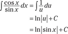
Combining the antiderivatives of each indefinite integral gives you the solution:

900. ![]()
Begin by expanding the integrand:
![]()
Next, use the identity ![]() to produce the following integral:
to produce the following integral:
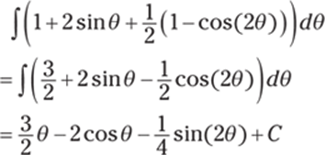
901. ![]()
Here's the given integral:
![]()
Begin by applying the identity sin(2x) = 2 sin x cos x to the denominator of the integrand. Then split up the fraction and simplify:
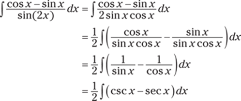
You can now apply basic antiderivative formulas to arrive at the solution:

902. ![]()
Here's the given integral:
![]()
Begin by rewriting the integral:
![]()
Then use the substitution u = tan x so that du = sec2 x dx:

903. ![]()
The given integral is
![]()
To integrate this function, use integration by parts: ![]() . Let u = x so that du = dx and let dv = sin2 x. Note that to find v by integrating dv, you have to use a trigonometric identity:
. Let u = x so that du = dx and let dv = sin2 x. Note that to find v by integrating dv, you have to use a trigonometric identity:
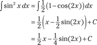
Therefore, you get the following:

904. ![]()
Here's the given integral:
![]()
For this problem, you can factor out either sin x or cos x and then use an identity. For example, you can factor out cos x and then use the identity cos2 x = 1 – sin2 x:

Then use the substitution u = sin x so that du = cos x dx to get
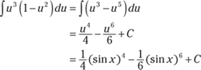
905. ![]()
The given integral is
![]()
Begin by factoring out tan x and using an identity:
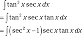
Now use the substitution u = sec x so that du = sec x tan x dx. This gives you

906. ![]()
Begin by factoring out cot x and using an identity:

Now use the substitution u = csc x so that du = –csc x cot x dx, or –du = csc x cot x dx. This gives you the following:

907. ![]()
Here's the given integral:
![]()
Begin by factoring out cos x and using a trigonometric identity to write cos2 x in terms of sin x:
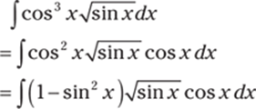
Now use u-substitution: u = sin x so that du = cos x. Using these values in the integral gives you
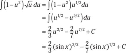
908. ![]()
Begin by factoring out ![]() and using an identity to get the following:
and using an identity to get the following:

Now use the substitution u = cot x so that du = –csc2 x dx, or –du = csc2 x dx:

909. ![]()
Here's the given integral:
![]()
Begin by performing the substitution ![]() so that
so that ![]() , or
, or ![]() . Using these values in the integral gives you
. Using these values in the integral gives you ![]() . Now factor out sin u and use some algebra and a trigonometric identity to write sin2 u in terms of cos u:
. Now factor out sin u and use some algebra and a trigonometric identity to write sin2 u in terms of cos u:
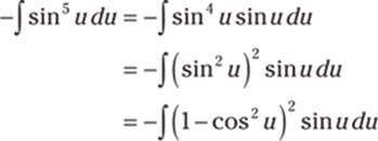
Again use a substitution to integrate: Let w = cos u so that dw = –sin u du, or –dw = sin u du. Using these values yields the integral ![]() . Now simply expand the integrand and integrate:
. Now simply expand the integrand and integrate:

Then undo all the substitutions:

910. ![]()
The given integral is
![]()
Begin by factoring out sin x and using a trigonometric identity to write sin2 x in terms of cos x:
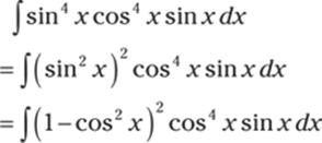
Now use the substitution u = cos x, which gives you du = –sin x dx, or –du = sin x dx. Using these values in the integral gives you
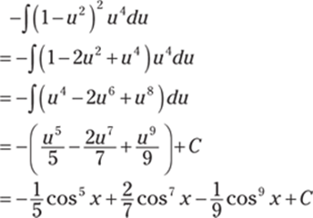
911. ![]()
To evaluate this integral, you can use integration by parts. You may want to first rewrite sec3 x as sec2 x sec x (rewriting isn't necessary, but it may help you see things a bit better!):
![]()
Now use integration by parts with u = sec x so that du = sec x tan x dx and let dv = sec2 x dx so that v = tan x. This gives you the following:

Now use an identity to get
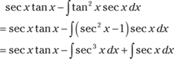
Set this expression equal to the given integral:
![]()
After evaluating ![]() on the right side of the equation, you get
on the right side of the equation, you get
![]()
Add ![]() to both sides of the equation and then divide by 2 to get the solution:
to both sides of the equation and then divide by 2 to get the solution:
![]()
912. –sec x – tan x + C
The given integral is
![]()
Begin by multiplying the numerator and denominator of the integrand by the conjugate of the denominator. Recall that the conjugate of (a – b) is (a + b). In this case, you multiply the numerator and denominator by (sin x + 1):

Now use the identity sin2 x – 1 = –cos2 x and split apart the fraction to further simplify the integrand:
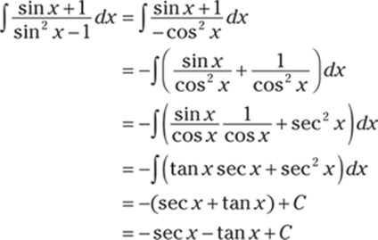
913. ![]()
Here's the given integral:
![]()
Begin by factoring out sec(4x) tan(4x):
![]()
Then use a trigonometric identity to arrive at
![]()
Now use the substitution u = sec(4x) so that du = 4 sec(4x) tan(4x) dx, or ![]() . Using these substitutions, you now have
. Using these substitutions, you now have
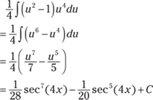
914. 
The given integral is

Start by using the substitution ![]() so that
so that ![]() . Using these substitutions in the integral, you get the following:
. Using these substitutions in the integral, you get the following:
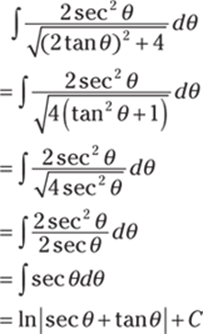
From the substitution ![]() , you get
, you get ![]() , from which you can deduce that
, from which you can deduce that ![]() . (To deduce that
. (To deduce that ![]() , you can label a right triangle using
, you can label a right triangle using ![]() and find the missing side using the Pythagorean theorem.) Using these values, you get
and find the missing side using the Pythagorean theorem.) Using these values, you get
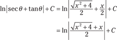
915. ![]()
Here's the given integral:

Begin by using the substitution ![]() so that
so that ![]() . You can find the newlimits of integration by noting that if
. You can find the newlimits of integration by noting that if ![]() , then
, then ![]() so that
so that ![]() , and if x = 0, then
, and if x = 0, then ![]() so that
so that ![]() :
:
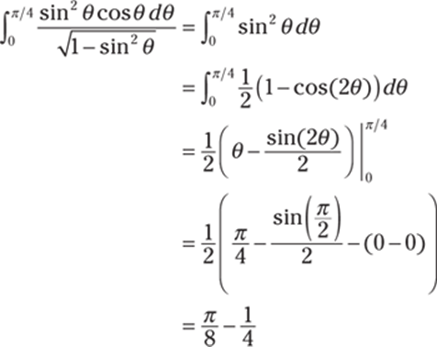
916. ![]()
Here's the given integral:
![]()
Use the trigonometric substitution ![]() so that
so that ![]() :
:
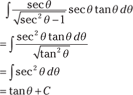
From ![]() , you can deduce that
, you can deduce that ![]() . (To deduce that
. (To deduce that ![]() , you can label a right triangle using
, you can label a right triangle using ![]() and then use the Pythagorean theoremto find the missing side.) Therefore, the solution becomes
and then use the Pythagorean theoremto find the missing side.) Therefore, the solution becomes
![]()
Note that you can also solve the problem with the substitution u = x2 – 1.
917. 
The given integral is

Begin with the trigonometric substitution ![]() to get
to get ![]() , which gives you the following:
, which gives you the following:
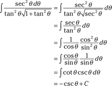
From ![]() , you can deduce that
, you can deduce that  . (To deduce that
  ,you can label a right triangle using
 ![]() and then find the missing side using thePythagorean theorem.) Therefore, you get the following solution:
and then find the missing side using thePythagorean theorem.) Therefore, you get the following solution:

918. 
The given integral is

Begin by using the substitution ![]() to get
to get ![]() . Substituting these values into the original integral, you have
. Substituting these values into the original integral, you have
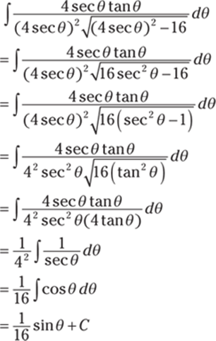
From your original substitution, you have ![]() . From this, you can deduce that
. From this, you can deduce that  . (To deduce that
  , you can label a right triangle using
 ![]() and then use the Pythagorean theorem to find the missing side.) Therefore, the solution becomes
and then use the Pythagorean theorem to find the missing side.) Therefore, the solution becomes

919. 
Here's the given integral:
![]()
Begin by using the trigonometric identity ![]() so that
so that ![]() :
:
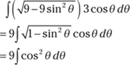
Now use an identity to get
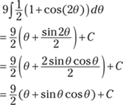
From the substitution ![]() , you get
, you get ![]() , so you can deduce that
, so you can deduce that ![]() and that
and that  . (To deduce that
  , you can label a right triangle using
 ![]() and then find the missing side with the Pythagorean theorem.) Therefore, the solution becomes
and then find the missing side with the Pythagorean theorem.) Therefore, the solution becomes
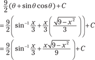
920. ![]()
Start by rewriting the given integral:
![]()
Now you can use the substitution ![]() to get
to get ![]() and
and ![]() . Substituting these values into the integral, you get
. Substituting these values into the integral, you get
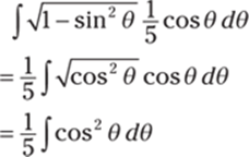
Then you can use the identity ![]() to simplify the integral:
to simplify the integral:
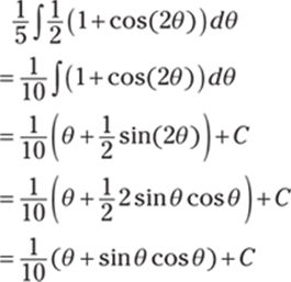
From the substitution ![]() , you can deduce that
, you can deduce that ![]() and also that
and also that ![]() . (To deduce that
. (To deduce that ![]() , you can label a right triangle using
, you can label a right triangle using ![]() and find the missing side of the triangle with the Pythagorean theorem.) Using these values, you get the solution:
and find the missing side of the triangle with the Pythagorean theorem.) Using these values, you get the solution:

921. 
The given integral is

Begin by using the substitutions ![]() and
and ![]() :
:
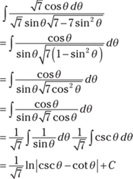
From the substitution ![]() , you get
, you get ![]() , from which you can deduce that
, from which you can deduce that ![]() and also that
and also that  . (To deduce that
  , you can label a right triangle using
 ![]() and find the missing side of the triangle with the Pythagorean theorem.) Using these values, you get the following solution:
and find the missing side of the triangle with the Pythagorean theorem.) Using these values, you get the following solution:

922. ![]()
Rewrite the integral with a radical sign:
![]()
Now begin by using the substitution ![]() , or
, or ![]() , so that
, so that ![]() :
:
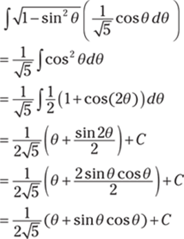
From the substitution ![]() , you can deduce that
, you can deduce that ![]() and that
and that ![]() . (To deduce that
. (To deduce that ![]() , you can label a right triangle using
, you can label a right triangle using ![]() and find the missing side of the triangle with the Pythagorean theorem.) Therefore, the solution becomes
and find the missing side of the triangle with the Pythagorean theorem.) Therefore, the solution becomes

923. 
The given integral is

Begin by using the trigonometric substitution ![]() so that
so that ![]() :
:
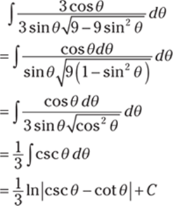
From the substitution ![]() , you can deduce that
, you can deduce that ![]() and that
and that  . (To deduce that
  , you can label a right triangle using
 ![]() and find the missing side of the triangle with the Pythagorean theorem.) Therefore, the solution becomes
and find the missing side of the triangle with the Pythagorean theorem.) Therefore, the solution becomes

924. 
The given integral is

Begin with the trigonometric substitution ![]() so that
so that ![]() :
:
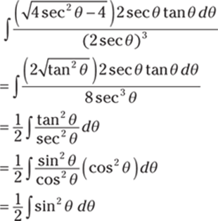
Now use an identity to get
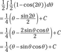
From the substitution ![]() , you can deduce that
, you can deduce that ![]() ,
,  , and
, and ![]() . (To find the values of
. (To find the values of ![]() and
and ![]() , you can label a right triangle using
, you can label a right triangle using ![]() and find the missing side of the triangle with the Pythagorean theorem.) Therefore, the solution becomes
and find the missing side of the triangle with the Pythagorean theorem.) Therefore, the solution becomes
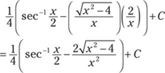
925. ![]()
The given integral is
![]()
Begin with the substitution u = x2 so that du = 2x dx, or ![]() :
:
![]()
Now use the substitution ![]() so that
so that ![]() :
:
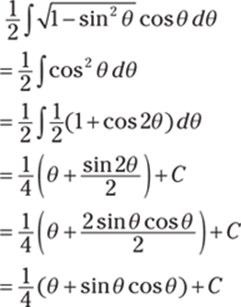
From the substitution ![]() , you can deduce that
, you can deduce that ![]() and that
and that ![]() . Therefore, the answer is
. Therefore, the answer is
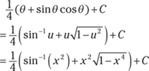
926. ![]()
Here's the given integral:

First begin with the substitution u = cos t, which gives you du = –sin t dt, or –du = sin t dt. You can also compute the new limits of integration: If ![]() , then
, then ![]() , and if t = 0, then u = cos 0 = 1. Substituting these values into the integral gives you
, and if t = 0, then u = cos 0 = 1. Substituting these values into the integral gives you

Next, use the trigonometric substitution ![]() , which gives you
, which gives you ![]() . You can again find the new limits of integration: If u = 1, then
. You can again find the new limits of integration: If u = 1, then ![]() so that
so that ![]() , and if u = 0, then
, and if u = 0, then ![]() so that
so that ![]() . Using these values, you produce the integral
. Using these values, you produce the integral

Now use a trigonometric identity and simplify:
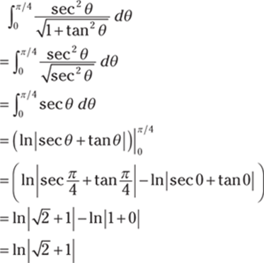
927. ![]()
Here's the given integral:

Begin with the substitution ![]() so that
so that ![]() :
:
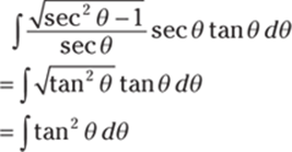
Next, use an identity and integrate to get
![]()
From the substitution ![]() , you can deduce that
, you can deduce that ![]() and that
and that ![]() to get the solution:
to get the solution:
![]()
928. ![]()
The given integral is

Use the trigonometric substitution ![]() so that
so that ![]() . You can find the new limits of integration by noting that if x = 1, then
. You can find the new limits of integration by noting that if x = 1, then ![]() and
and ![]() and that if x = 2, then
and that if x = 2, then ![]() and
and ![]() . With these new values, you get
. With these new values, you get
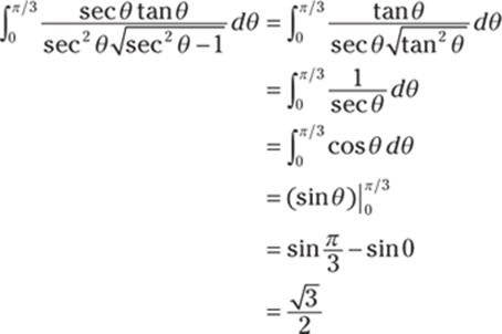
929. 
Start by rewriting the denominator with a radical:

Use the trigonometric substitution ![]() to get
to get ![]() . These substitutions give you the following:
. These substitutions give you the following:
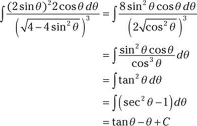
From the substitution ![]() , or
, or ![]() , you can deduce that
, you can deduce that ![]() and that
and that ![]() . (To deduce that
. (To deduce that ![]() , you can label a right triangle using
, you can label a right triangle using ![]() and then find the missing side with the Pythagorean theorem.) Therefore, the solution becomes
and then find the missing side with the Pythagorean theorem.) Therefore, the solution becomes

930. 
Start by rewriting the integrand:

Use the substitution ![]() , or
, or ![]() , so that
, so that ![]() :
:
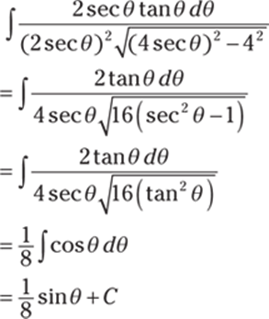
From ![]() , or
, or ![]() , you can deduce that
, you can deduce that  . (To deduce that
  , you can label a right triangle using
 ![]() and then find the missing side of the triangle with the Pythagorean theorem.) Therefore, the solution becomes
and then find the missing side of the triangle with the Pythagorean theorem.) Therefore, the solution becomes

931. 
Here's the given integral:

Begin with the substitution ![]() to get
to get ![]() . Substituting this value into the original integral gives you the following:
. Substituting this value into the original integral gives you the following:
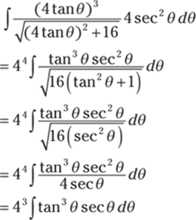
Now factor out ![]() and use a trigonometric identity along with a u-substitution:
and use a trigonometric identity along with a u-substitution:

Let ![]() to get
to get ![]() . Using these values in the integral, you get
. Using these values in the integral, you get

From the first substitution, you get ![]() , from which you can deduce that
, from which you can deduce that ![]() . (You can find the value
. (You can find the value ![]() by using a trigonometric identity for tangent and secant.) Inserting this value into the preceding equation and simplifying a bit gives you the answer:
by using a trigonometric identity for tangent and secant.) Inserting this value into the preceding equation and simplifying a bit gives you the answer:
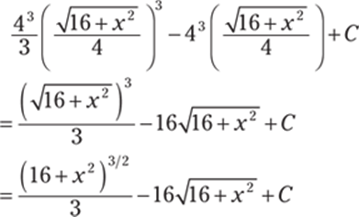
932. ![]()
Here's the given integral:

Begin with the substitution ![]() so that
so that ![]() :
:

Next, use an identity to get

Now use the substitution ![]() so that
so that ![]() :
:
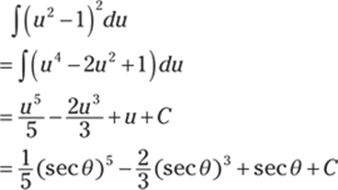
From the substitution ![]() , you can deduce that
, you can deduce that ![]() to get the solution:
to get the solution:

Note that you can also do this problem starting with the substitution ![]() and a bit of algebra.
and a bit of algebra.
933. 
The given expression is
![]()
Let ![]() to get
to get ![]() . You can also find the new limits of integration by using the original limits along with the substitution
. You can also find the new limits of integration by using the original limits along with the substitution ![]() . If x = 3, you get
. If x = 3, you get ![]() , or
, or ![]() , so that
, so that ![]() . Likewise, if x = 0, you get
. Likewise, if x = 0, you get ![]() , or
, or ![]() , so that
, so that ![]() . Using these substitutions and the new limits of integration gives you the following:
. Using these substitutions and the new limits of integration gives you the following:
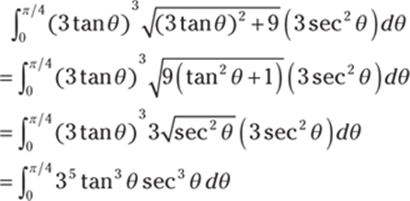
Now factor out ![]() and use a trigonometric identity:
and use a trigonometric identity:
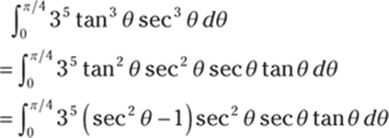
Use the substitution ![]() so that
so that ![]() . You can again find the new limits of integration; with
. You can again find the new limits of integration; with ![]() , you get
, you get ![]() , and with
, and with ![]() , you get u = sec 0 = 1. Using the new limits and the substitution, you can get the answer as follows:
, you get u = sec 0 = 1. Using the new limits and the substitution, you can get the answer as follows:
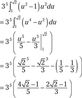
934. ![]()
Start by rewriting the integrand:
![]()
Use a substitution, letting w = x3, to get dw = 3x2 dx, or ![]() . Putting these values into the integral gives you
. Putting these values into the integral gives you
![]()
Now use the trigonometric substitution ![]() , which gives you
, which gives you ![]() . Using these values in the integral gives you the following:
. Using these values in the integral gives you the following:
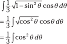
Now you can use the identity ![]() to rewrite the integral:
to rewrite the integral:
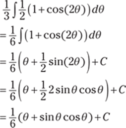
From ![]() , you can deduce that
, you can deduce that ![]() and that
and that ![]() . (Note that you can find the value for
. (Note that you can find the value for ![]() by using an identity for sine and cosine.) Substituting these values into the integral gives you
by using an identity for sine and cosine.) Substituting these values into the integral gives you
![]()
Replacing w with x3 gives you the solution:
![]()
935. 
Rewrite the denominator as a radical:

Now you complete the square on the quadratic expression:
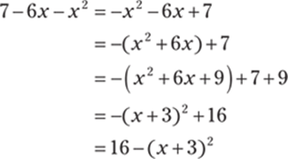
So the integral becomes

Now use the substitution ![]() , which gives you
, which gives you ![]() . Substituting these values into the integral gives you
. Substituting these values into the integral gives you
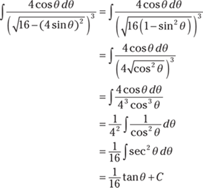
From the substitution ![]() , or
, or ![]() , you can deduce that
, you can deduce that  . (To deduce that
  , you can label a right triangle using
 ![]() and then find the missing side with the Pythagorean theorem.) Therefore, the solution is
and then find the missing side with the Pythagorean theorem.) Therefore, the solution is

936. 
Here's the given integral:
![]()
This may not look like a trigonometric substitution problem at first glance because so many of those problems involve some type of radical. However, many integrals that contain quadratic expressions can still be solved with this method.
First complete the square on the quadratic expression:
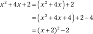
So the integral becomes

Use the substitution ![]() , which gives you
, which gives you ![]() . Putting this value into your integral yields
. Putting this value into your integral yields
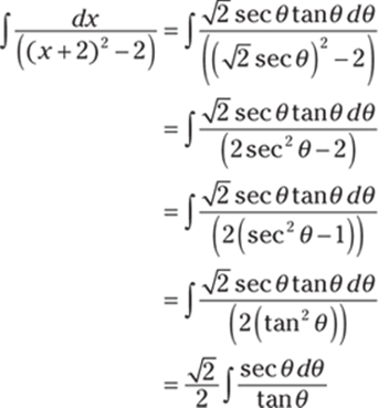
Because ![]() , you have
, you have

From the substitution ![]() , or
, or  , you can deduce that
  and that
  . (To deduce these values for
 ![]() and
and ![]() , you can label a right triangle using
, you can label a right triangle using  and then find the missing side using the Pythagorean theorem.) Putting these values into the antiderivative gives you the solution:
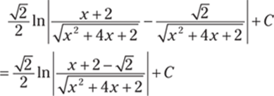
937. ![]()
You can begin by rewriting the expression underneath of the radical to make the required substitution clearer:
![]()
Use the substitution ![]() to get
to get ![]() so that
so that ![]() . You can find the new limits of integration by using the original limits of integration and the substitution. If
. You can find the new limits of integration by using the original limits of integration and the substitution. If ![]() , then
, then ![]() , or
, or ![]() , so that
, so that ![]() . Likewise, if x = 0, then
. Likewise, if x = 0, then ![]() so that
so that ![]() , or
, or ![]() . Using this information, you can produce the following integral:
. Using this information, you can produce the following integral:
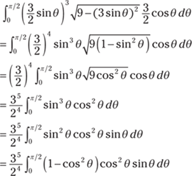
Now use the substitution ![]() so that
so that ![]() , or
, or ![]() . You can again find the new limits of integration: If
. You can again find the new limits of integration: If ![]() , then
, then ![]() . Likewise, if
. Likewise, if ![]() , then u = cos 0 = 1. Using the substitution along with the new limits of integration, you get the following (recall that when you switch the limits of integration, the sign on the integral changes):
, then u = cos 0 = 1. Using the substitution along with the new limits of integration, you get the following (recall that when you switch the limits of integration, the sign on the integral changes):
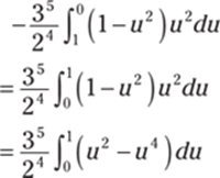
Now you have the following:
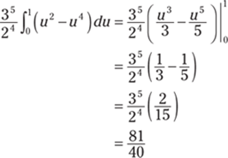
938. 
Here's the given integral:
![]()
First complete the square on the quadratic expression underneath the square root:
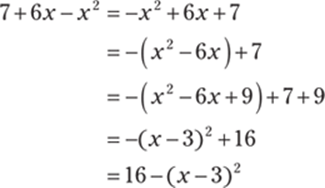
Therefore, you have the integral
![]()
Now you can use the substitution ![]() , which gives you
, which gives you ![]() . Substituting these values into the integral gives you
. Substituting these values into the integral gives you
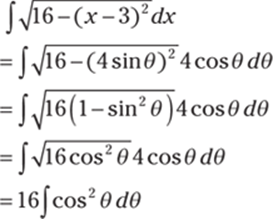
Then use the identity ![]() to simplify the integral:
to simplify the integral:
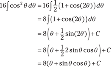
From the substitution ![]() , you get
, you get ![]() and
and ![]() . You can deduce that
. You can deduce that ![]() by labeling a right triangle using
by labeling a right triangle using ![]() and then finding the missing side of the triangle with the Pythagorean theorem. Putting these values into the antiderivative gives you the solution:
and then finding the missing side of the triangle with the Pythagorean theorem. Putting these values into the antiderivative gives you the solution:

939. ![]()
Here's the given integral:
![]()
Start with the substitution ![]() so that
so that ![]() . Substituting these values into the original integral, you get the following:
. Substituting these values into the original integral, you get the following:
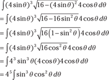
Now factor out ![]() and use a trigonometric identity along with a u-substitution:
and use a trigonometric identity along with a u-substitution:

With ![]() , you get
, you get ![]() , or
, or ![]() . Substituting these values into the integral gives you
. Substituting these values into the integral gives you
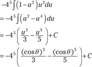
From the original substitution, you have ![]() , from which you can deduce that
, from which you can deduce that ![]() . (To deduce that
. (To deduce that ![]() , you can label a right triangle using
, you can label a right triangle using ![]() and then find the missing side with the Pythagorean theorem.) With these values, you arrive at the following solution:
and then find the missing side with the Pythagorean theorem.) With these values, you arrive at the following solution:
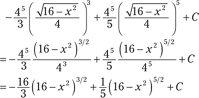
940. ![]()
The given expression is
![]()
Notice that you have the linear factor x raised to the third power and the linear factor (x + 1) raised to the second power. Therefore, in the decomposition, all the numerators will be constants:
![]()
941. ![]()
The given expression is
![]()
Begin by factoring the denominator completely:

In this expression, you have two distinct linear factors and one irreducible quadratic factor. Therefore, the fraction decomposition becomes

942. 
Here's the given expression:

In this expression, a linear factor is being squared, and an irreducible quadratic factor is raised to the third power. Therefore, the fraction decomposition becomes

943. 
The given expression is

In this example, you have the linear factor x that's being squared, the linear factor (x – 1) that's being cubed, and the irreducible quadratic factor (x2 + 17). Therefore, the fraction decomposition becomes

944. 
Begin by factoring the denominator of the expression:

In the expression on the right side of the equation, you have the distinct linear factors (x – 3) and (x + 3) and the irreducible quadratic factor (x2 + 1) that's being squared. Therefore, the fraction decomposition becomes

945. 
Start by performing the decomposition:
![]()
Multiply both sides of the equation by (x + 2)(x – 1):

Now let x = 1 to get 1 = A(1 – 1) + B(1 + 2) so that 1 = 3B, or ![]() . Also let x = –2 to get 1 = A(–2 – 1) + B(–2 + 2) so that 1 = –3A, or
. Also let x = –2 to get 1 = A(–2 – 1) + B(–2 + 2) so that 1 = –3A, or ![]() . Therefore, you arrive at
. Therefore, you arrive at

946. ![]()
Start by factoring the denominator:

Then perform the decomposition:

Multiply both sides of the equation by x(x2 + 1):

Note that if x = 0, then ![]() so that 2 = A. Next, expand the right side of the equation and equate the coefficients to find the remaining coefficients:
so that 2 = A. Next, expand the right side of the equation and equate the coefficients to find the remaining coefficients:
![]()
After rearranging, you get
![]()
Now equate coefficients to arrive at the equation 0 = A + B; however, you know that 2 = A, so 0 = 2 + B, or –2 = B. Likewise, by equating coefficients, you immediately find that C = 1. Therefore, the partial fraction decomposition becomes

947. 
Start by factoring the denominator:

Then perform the fraction decomposition:

Multiply both sides of the equation by (x – 3)2:

By letting x = 3 in the last equation, you arrive at 5(3) + 1 = A(3 – 3) + B, so 16 = B. By expanding the right side of the equation, you get
![]()
So by equating coefficients, you immediately see that 5 = A. Therefore, the fraction decomposition becomes

948. 
Begin by factoring the denominator:

Then perform the decomposition:

Multiply both sides of the equation by (x2 + 1)(x2 + 3) to get
![]()
Expand the right side of the equation and collect like terms:

Equating coefficients gives you the equations A + C = 0, B + D = 1, 3A + C = 0, and 3B + D = 2. Because A = –C, you get 3(–C) + C = 0, so –2C = 0, or C = 0; that means A = 0 as well. Likewise, because B = 1 – D, you get 3(1 – D) + D = 2, so 3 – 2D = 2, or ![]() ; you also get
; you also get ![]() . With these values, you get the following solution:
. With these values, you get the following solution:
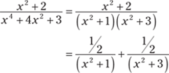
949. 
Begin by performing the decomposition:

Multiplying both sides of the equation by (x2 + 5)2 gives you

Expand the right side of the equation and regroup:

By equating coefficients, you find A = 0, B = 1, 5A + C = 0, and 5B + D = 0. Using A = 0 and 5A + C = 0, you get 5(0) + C = 0, or C = 0. Likewise, using B = 1 and 5B + D = 1, you find that 5(1) + D = 1 so that D = –4. Therefore, the fraction decomposition becomes
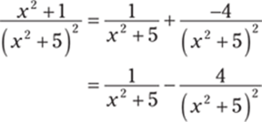
950. ![]()
The given integral is
![]()
Notice that the degree of the numerator is equal to the degree of the denominator, so you must divide. You could use long division, but for simple expressions of this type, you can simply subtract 5 and add 5 to the numerator and then split the fraction:
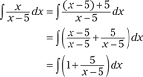
Now apply elementary antiderivative formulas to get the solution:
![]()
951. ![]()
The given integral is
![]()
The degree of the numerator is greater than or equal to the degree of the denominator, so use polynomial long division to get the following:
![]()
Then apply basic antiderivative formulas:
![]()
952. ![]()
The given integral is
![]()
First perform a fraction decomposition on the integrand:
![]()
Multiplying both sides of the equation by (x + 4)(x – 5) and simplifying gives you

Now you can find the values of the coefficients by picking appropriate values of x and solving the resulting equations. So if you let x = 5, you get 5 – 3 = A(5 – 5) + B(5 + 4), or 2 = 9B, so that ![]() . Likewise, if x = –4, then you get –4 – 3 = A(–4 – 5) + B(–4 + 4), or –7 = A(–9), so that
. Likewise, if x = –4, then you get –4 – 3 = A(–4 – 5) + B(–4 + 4), or –7 = A(–9), so that ![]() . This gives you
. This gives you
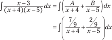
Applying elementary antiderivative formulas gives you the solution:
![]()
953. 
The given expression is
![]()
First factor the denominator of the integrand:
![]()
Then perform the fraction decomposition:
![]()
Multiplying both sides of the equation by (x + 1)(x – 1) and simplifying gives you

Now you can solve for the coefficients by picking appropriate values of x. Notice that if x = 1, you get 1 = A(1 – 1) + B(1 + 1) so that 1 = 2B, or ![]() . Likewise, if x = –1, you get 1 = A(–1 – 1) + B(–1 + 1) so that 1 = –2A, or
. Likewise, if x = –1, you get 1 = A(–1 – 1) + B(–1 + 1) so that 1 = –2A, or ![]() . This gives you
. This gives you
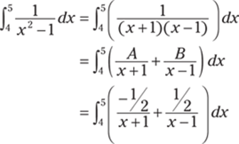
Applying elementary antiderivatives gives you the following:
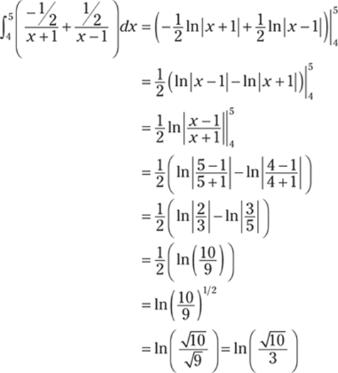
954. ![]()
The given integral is
![]()
Begin by factoring the denominator:

And then perform a fraction decomposition:

Multiplying both sides by (x + 1)2 gives you the following:

Expanding the right side and equating coefficients gives you 3x + 5 = Ax + (A + B) so that A = 3 and A + B = 5; in turn, that gives you 3 + B = 5 so that B = 2. Now you have
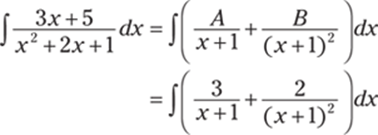
For the first term in the integrand, simply use an elementary antiderivative:
![]() . For the second term in the integrand, use a substitution on
. For the second term in the integrand, use a substitution on ![]() where u = x + 1 so that du = dx. Using these values gives you
where u = x + 1 so that du = dx. Using these values gives you
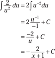
Therefore, the answer is

Note: You can also evaluate  with the substitution u = x + 1 so that du = dx and u – 1 = x.
955. ![]()
The given expression is
![]()
The degree of the numerator is greater than or equal to the degree of the denominator, so use polynomial long division to get the following:

Next, perform a fraction decomposition:
![]()
Multiply both sides of the equation by (x – 3)(x + 2):
![]()
If you let x = 2, you get 9 = B(–2 – 3) so that ![]() . And if you let x = 3, you get 14 = A(3 + 2) so that
. And if you let x = 3, you get 14 = A(3 + 2) so that ![]() . With these values, you produce the following integral:
. With these values, you produce the following integral:

To integrate, use basic antiderivative formulas to get

956. ![]()
The given expression is
![]()
First factor the denominator of the integrand:

And then perform the fraction decomposition:

Multiply both sides by x(x2 + 1) and simplify to get

Expanding the right side, rearranging terms, and rewriting the left side yields the following:

Equating coefficients gives you 0 = A + B, 0 = C, and 8 = A. Using 8 = A and 0 = A + B gives you 0 = 8 + B, or –8 = B. These values give you the following integral:
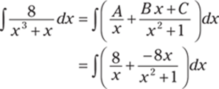
To evaluate the first term in the integrand, use elementary antiderivatives:
![]() . To evaluate the second term in the integrand, use a substitution on
. To evaluate the second term in the integrand, use a substitution on ![]() where u = x2 + 1 so that du = 2x dx. Multiplying both sides of last equation by –4 gives you –4 du = –8x dx. Using these substitutions gives you the following:
where u = x2 + 1 so that du = 2x dx. Multiplying both sides of last equation by –4 gives you –4 du = –8x dx. Using these substitutions gives you the following:
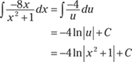
Combining the two antiderivatives gives you the solution:

957. 
The given expression is
![]()
Begin by factoring the denominator of the integrand:

And do a fraction decomposition:

Multiply both sides by (x2 + 3)2 and simplify:

Expanding the right side, rearranging and collecting like terms, and rewriting the left side gives you

Equating coefficients gives you A = 0, B = 6, 3A + C = 0, and 3B + D = 1. Using 3B + D = 1 and B = 6 gives you 3(6) + D = 1, or D = –17. From A = 0 and 3A + C = 0, you can conclude that C = 0. So the original integral becomes
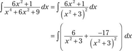
To integrate the first term in the integrand, simply use an elementary antiderivative formula:
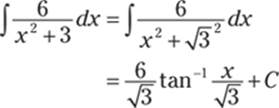
Integrating the second term of the integrand is a bit more difficult. Begin by using a trigonometric substitution:  with
with ![]() so that
so that ![]() . Using these substitutions gives you the following:
. Using these substitutions gives you the following:
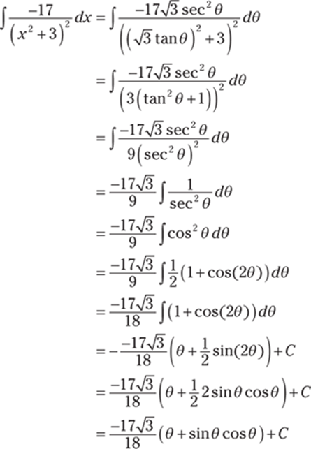
Using the substitution ![]() gives you
gives you ![]() , from which you can deduce that
, from which you can deduce that  ,
, ![]() , and
, and  .
.
So the antiderivative of the second term becomes
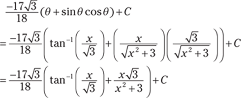
Combining the two solutions gives you the answer:
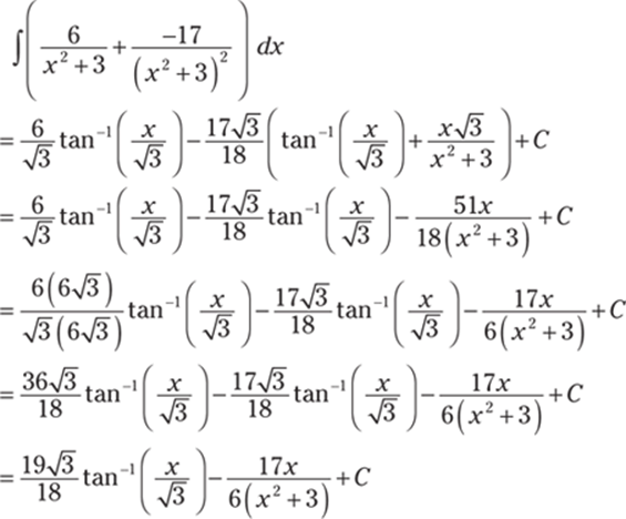
958. 
Begin by factoring the denominator:

Then find the fraction decomposition:

Multiply both sides by (x + 1)(x2 – x + 1), which yields
![]()
Expanding the right side and collecting like terms gives you

Equating coefficients gives you the equations 0 = A + B, 0 = –A + B + C, and 1 = A + C. From the first of the three equations, you have A = –B, and from the third, you get 1 – A = C so that 1 + B = C. Using the equation 0 = –A + B + C with A = –B and with 1 + B = C gives you 0 = –(–B) + B + (1 + B) so that ![]() ; therefore,
; therefore, ![]() and
and ![]() . With these coefficients, you now have the following integral:
. With these coefficients, you now have the following integral:

Next, complete the square on the expression x2 – x + 1:
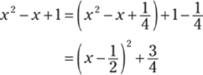
Splitting up the integral gives you

Using the substitution ![]() , you get du = dx and
, you get du = dx and ![]() so that
so that ![]() and
and ![]() . Using these values gives you
. Using these values gives you
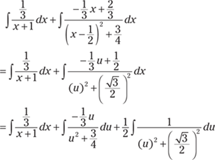
To evaluate the second integral,  , use the substitution
 ![]() so that dw = 2u du, or
so that dw = 2u du, or ![]() . This substitution gives you
. This substitution gives you
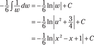
Therefore, the solution is
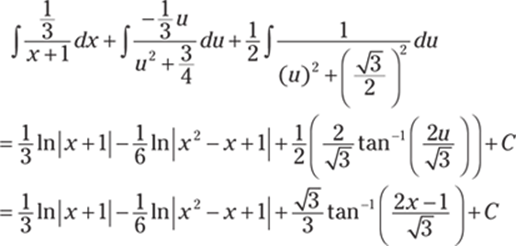
959. 
Here's the given problem:
![]()
Begin by using the rationalizing substitution ![]() so that u2 = x + 1, or u2 – 1 = x, and 2u du = dx. This substitution gives you
so that u2 = x + 1, or u2 – 1 = x, and 2u du = dx. This substitution gives you

Next, find the fraction decomposition:
![]()
Multiply both sides by (u – 1)(u + 1):
![]()
Notice that if u = –1, you get 1 = B(–2) so that ![]() , and if u = 1, you get 1 = A(2) so that
, and if u = 1, you get 1 = A(2) so that ![]() . With these values, you get the following:
. With these values, you get the following:
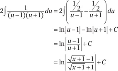
960. ![]()
Here's the given expression:
![]()
Begin by using the rationalizing substitution ![]() so that u2 = x and 2u du = dx. Note that if x = 9, you have
so that u2 = x and 2u du = dx. Note that if x = 9, you have ![]() , and if x = 4, you have
, and if x = 4, you have ![]() , producing the following integral:
, producing the following integral:

Next, perform the fraction decomposition:
![]()
And multiply both sides by (u – 1)(u + 1) to get
![]()
Notice that if u = –1, you get 1 = B(–2) so that ![]() , and if u = 1, you get 1 = A(2) so that
, and if u = 1, you get 1 = A(2) so that ![]() . With these values, you get the following:
. With these values, you get the following:
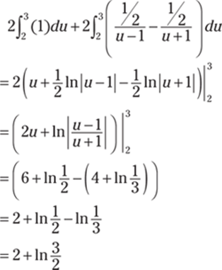
961. 
The given expression is
![]()
Begin by using the substitution ![]() so that u6 = x and 6u5 du = dx. Also notice that u2 = x1/3 and that u3 = x1/2. With these values, you produce the following integral:
so that u6 = x and 6u5 du = dx. Also notice that u2 = x1/3 and that u3 = x1/2. With these values, you produce the following integral:
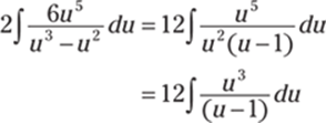
Because the degree of the numerator is greater than or equal to the degree of the denominator, use polynomial long division to get

Now use elementary antiderivative formulas to get the solution:
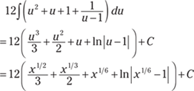
962. 
The given problem is
![]()
Begin by using the substitution ![]() so that u12 = x and so that 12u11 du = dx. Also notice that u4 = x1/3 and that u3 = x1/4. With these values, you produce the integral
so that u12 = x and so that 12u11 du = dx. Also notice that u4 = x1/3 and that u3 = x1/4. With these values, you produce the integral
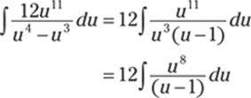
Because the degree of the numerator is greater than or equal to the degree of the denominator, use polynomial long division:

Then use elementary antiderivative formulas to get the answer:

963. 
The given expression is
![]()
Begin with the substitution u = ex so that du = ex dx:
![]()
Then perform the fraction decomposition:
![]()
Multiplying both sides by (u + 1)(u + 2) gives you u = A(u + 2) + B(u + 1). If you let u = –2, you get –2 = B(–2 + 1) so that 2 = B, and if u = –1, you get –1 = A(–1 + 2) so that –1 = A. With these values, you have
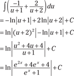
964. convergent, ![]()
Begin by rewriting the integral using a limit:
![]()
First evaluate ![]() using the substitution u = x + 1 so that du = dx. Using these substitutions gives you
using the substitution u = x + 1 so that du = dx. Using these substitutions gives you
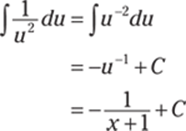
Because ![]() , you have the following after replacing the limit at infinity and the limits of integration:
, you have the following after replacing the limit at infinity and the limits of integration:

Now evaluate the limit:
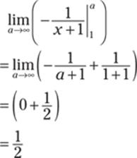
Because the value of the integral is finite, the improper integral is convergent.
965. divergent
Note that the function ![]() has an infinite discontinuity when x = 0, which is included in the interval of integration, so you have an improper integral. Begin by rewriting the definite integral using limits; then integrate:
has an infinite discontinuity when x = 0, which is included in the interval of integration, so you have an improper integral. Begin by rewriting the definite integral using limits; then integrate:
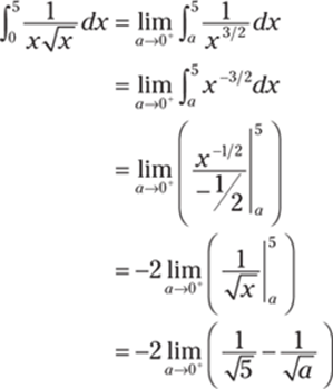
Because ![]() , you can conclude that
, you can conclude that ![]() is divergent.
is divergent.
966. divergent
Note that the function ![]() has an infinite discontinuity when x = 0, which is included in the interval of integration, so you have an improper integral. Begin by rewriting the definite integral using limits; then integrate:
has an infinite discontinuity when x = 0, which is included in the interval of integration, so you have an improper integral. Begin by rewriting the definite integral using limits; then integrate:
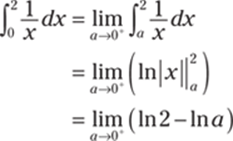
Because ![]() , you know that
, you know that ![]() is divergent.
is divergent.
967. divergent
Begin by rewriting the integral using a limit:
![]()
Then use elementary antiderivatives to get the following:
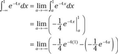
Because ![]() , the integral is divergent.
, the integral is divergent.
968. convergent, ![]()
Notice that the function f (x) = (x – 1)−1/4 has an infinite discontinuity when x = 1, which is included in the interval of integration, so you have an improper integral. Begin by writing the integral using a limit:
![]()
Notice that  so that

Substituting in the limits of integration and evaluating the limit gives you
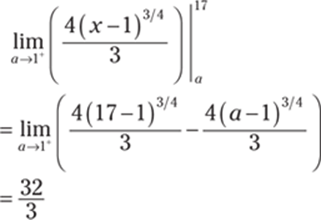
The answer is finite, so the integral is convergent.
969. divergent
Begin by rewriting the integral using a limit:
![]()
To evaluate this integral, use elementary antiderivatives:
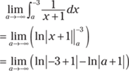
Because ![]() , the integral is divergent.
, the integral is divergent.
970. divergent
Begin by rewriting the improper integral using a definite integral and a limit; then integrate:
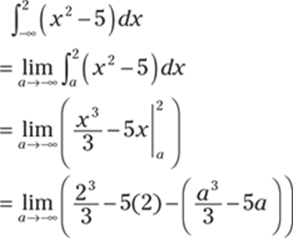
Notice that  . Because the first term in the numerator is the dominant term, you have

Therefore, it follows that

and you can conclude the integral is divergent.
971. divergent
Begin by splitting up the integral into two separate integrals, using limits to rewrite each integral:

Evaluate the first integral by integrating; then evaluate the resulting limit:
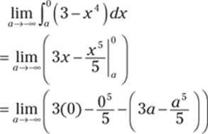
Notice that  . Because the second term in the numerator is the dominant term, you have

Therefore, it follows that

and you can conclude that the integral is divergent. Because the first integral is divergent, you don't need to evaluate the second integral; ![]() is divergent.
is divergent.
972. convergent, ![]()
Begin by rewriting the integral using a limit:
![]()
To evaluate ![]() , let
, let ![]() so that
so that ![]() , or –3 du = dx. This gives you
, or –3 du = dx. This gives you
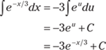
Because ![]() , it follows that
, it follows that
![]()
Now simply evaluate the limit:
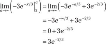
The answer is finite, so the integral is convergent.
973. convergent, 1
Begin by writing the integral using a limit:
![]()
To evaluate ![]() , use the substitution u = ln x so that
, use the substitution u = ln x so that ![]() :
:
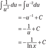
Because ![]() , it follows that
, it follows that

Evaluating the limit gives you
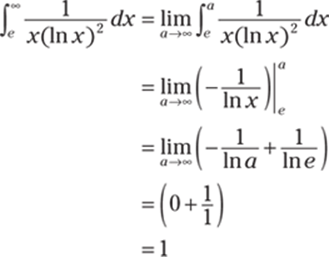
The answer is finite, so the integral is convergent.
974. convergent, ![]()
Begin by splitting the integral into two integrals, using limits to rewrite each integral:

To evaluate ![]() , rewrite the integral as
, rewrite the integral as  . Then use a substitution, letting u = x3 so that du = 3x2 dx, or
 ![]() . Using these substitutions gives you
. Using these substitutions gives you
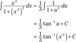
Therefore, as a approaches –∞, you have
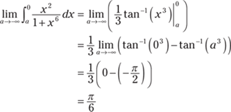
And as b approaches ∞, you have
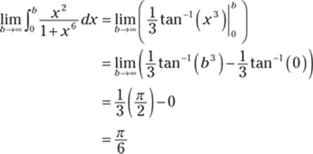
Combining the two values gives you the answer:
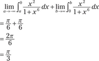
The answer is finite, so the integral is convergent.
Note: If you noticed that the integrand is even, you could've simply computed one of the integrals and multiplied by 2 to arrive at the solution.
975. convergent, ![]()
Begin by rewriting the integral using a limit:
![]()
To evaluate ![]() , use integration by parts. If u = x, then du = dx, and if dv = e−2x, then
, use integration by parts. If u = x, then du = dx, and if dv = e−2x, then ![]() :
:

Because ![]() , it follows that
, it follows that

Next, evaluate the limit:

Notice that ![]() and that
and that ![]() , which is an indeterminate form. To evaluate
, which is an indeterminate form. To evaluate ![]() , use L'Hôpital's rule:
, use L'Hôpital's rule:
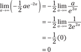
Using these values gives you

The answer is finite, so the integral is convergent.
976. divergent
Begin by splitting up the integral into two separate integrals, using limits to rewrite each integral:
![]()
To evaluate ![]() , use the substitution u = –x5 so that du = –5x4 dx, or
, use the substitution u = –x5 so that du = –5x4 dx, or ![]() :
:
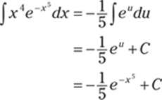
Because ![]() , it follows that
, it follows that

Next, evaluate the limit:

Notice that ![]() so that
so that ![]() is divergent. Because this integral is divergent, you don't need to evaluate
is divergent. Because this integral is divergent, you don't need to evaluate ![]() . You can conclude that
. You can conclude that ![]() is divergent.
is divergent.
977. convergent, ![]()
Begin by rewriting the integral using a limit:
![]()
To evaluate ![]() , rewrite the integral as
, rewrite the integral as  . Then use a substitution where u = x2 so that du = 2x dx, or
 ![]() :
:
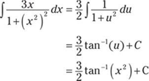
Because  , it follows that

Now evaluate the limit:
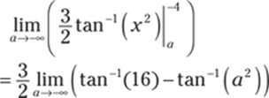
Notice that ![]() so that
so that

The answer is finite, so the integral is convergent.
978. convergent, ![]()
Begin by rewriting the integral using a limit:
![]()
To evaluate ![]() , use integration by parts. If u = ln x, then
, use integration by parts. If u = ln x, then ![]() , and if dv = x−4 dx, then
, and if dv = x−4 dx, then ![]() :
:
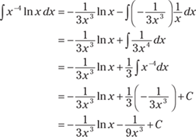
Because ![]() , it follows that
, it follows that

Evaluating the limit gives you
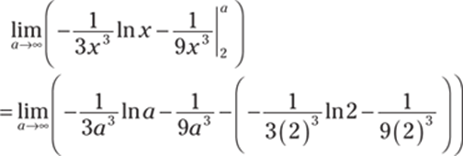
Notice that ![]() has the indeterminate form
has the indeterminate form ![]() , so you can use L'Hôpital's rule to evaluate it:
, so you can use L'Hôpital's rule to evaluate it:

Because ![]() , the limit becomes
, the limit becomes
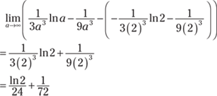
The answer is finite, so the integral is convergent.
979. divergent
Begin by rewriting the integral using a limit:
![]()
To find ![]() , let u = x2 + 4 so that du = 2x dx, or
, let u = x2 + 4 so that du = 2x dx, or ![]() . This substitution gives you
. This substitution gives you
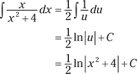
Because ![]() , you have
, you have

Evaluating the limit gives you

Therefore, the integral is divergent.
980. convergent, ![]()
Begin by rewriting the integral using a limit:
![]()
To evaluate ![]() , let u = x – 8 so that du = dx. This substitution gives you
, let u = x – 8 so that du = dx. This substitution gives you
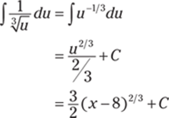
Because ![]() , you have
, you have

Evaluating the limit gives you
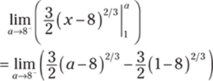
Noting that ![]() , you get the following:
, you get the following:
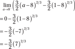
The answer is finite, so the integral is convergent.
981. divergent
Begin by rewriting the integral using a limit:

To evaluate ![]() , use a trigonometric identity:
, use a trigonometric identity:

Because ![]() , you have
, you have

Evaluating the limit gives you
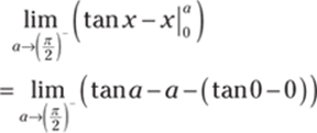
However, because  , you can conclude that
 ![]() is divergent.
is divergent.
982. divergent
Begin by rewriting the integral using a limit:
![]()
To evaluate ![]() , use the trigonometric identity
, use the trigonometric identity ![]() so that
so that

Because ![]() , it follows that
, it follows that

Evaluating the limit gives you

Because ![]() and because sin(2a) is always between –1 and 1, the integral is divergent.
and because sin(2a) is always between –1 and 1, the integral is divergent.
983. divergent
Notice that the function ![]() has an infinite discontinuity at x = 0. Rewrite the integral using limits:
has an infinite discontinuity at x = 0. Rewrite the integral using limits:
![]()
To evaluate ![]() , use the substitution u = ex – 1 so that du = ex dx to get
, use the substitution u = ex – 1 so that du = ex dx to get

Because ![]() , it follows that
, it follows that
![]()
Evaluating the limit gives you

However, because ![]() , the integral
, the integral ![]() is divergent, so you can conclude that
is divergent, so you can conclude that ![]() is divergent.
is divergent.
984. convergent, ![]()
Begin by writing the integral using a limit:
![]()
To evaluate ![]() , use a partial fraction decomposition:
, use a partial fraction decomposition:
![]()
Multiply both sides of the equation ![]() by (x + 3)(x – 2) to get
by (x + 3)(x – 2) to get
![]()
If you let x = 2, you have 1 = B(2 + 3) so that ![]() . And if x = –3, then 1 = A(–3 – 2) so that
. And if x = –3, then 1 = A(–3 – 2) so that ![]() . Entering these values, you get
. Entering these values, you get
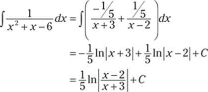
Because ![]() , it follows that
, it follows that

Evaluating the limit gives you
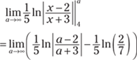
Because ![]() , you get the following solution:
, you get the following solution:
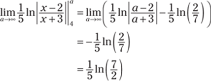
The answer is finite, so the integral is convergent.
985. convergent, ![]()
Begin by writing the integral using a limit:

To evaluate  , use the trigonometric substitution
 ![]() so that
so that ![]() . This gives you
. This gives you
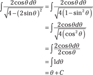
From the substitution ![]() , or
, or ![]() , you have
, you have ![]() ; therefore,
; therefore,
![]()
Because  , it follows that

Evaluating the limit gives you
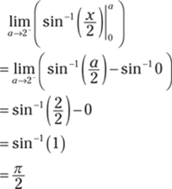
The answer is finite, so the integral is convergent.
986. convergent, 2
Rewrite the integral using limits:
![]()
On the interval (–∞, 0), you have ![]() , and on the interval (0, ∞), you have
, and on the interval (0, ∞), you have ![]() . Therefore, the limit is
. Therefore, the limit is
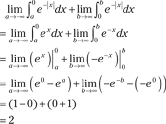
The answer is finite, so the integral is convergent.
987. convergent, ![]()
Begin by rewriting the integral using a limit:
![]()
To evaluate ![]() , let u = x – 3 so that u – 3 = x and du = dx. This gives you
, let u = x – 3 so that u – 3 = x and du = dx. This gives you
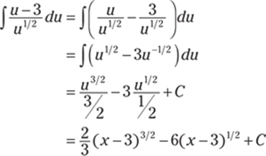
Because ![]() , it follows that
, it follows that

Substitute in the limits of integration and evaluate the resulting limit:
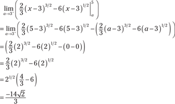
The answer is finite, so the integral is convergent.
988. convergent, compare to ![]()
Recall the comparison theorem: Suppose that f and g are continuous functions with f (x) ≥ g(x) ≥ 0 for x ≥ a.
· If ![]() is convergent, then
is convergent, then ![]() is convergent.
is convergent.
· If ![]() is divergent, then
is divergent, then ![]() is divergent.
is divergent.
The given improper integral is ![]() . Notice that on the interval [1, ∞], the following inequalities are true: –1 ≤ sin x ≤ 1; therefore, 0 ≤ sin2 x ≤ 1. Because 1 + x2 ≥ 0, you have
. Notice that on the interval [1, ∞], the following inequalities are true: –1 ≤ sin x ≤ 1; therefore, 0 ≤ sin2 x ≤ 1. Because 1 + x2 ≥ 0, you have ![]() . However,
. However, ![]() on [1, ∞] so that
on [1, ∞] so that ![]() . An integral of the form
. An integral of the form ![]() converges if and only if p > 1, so
converges if and only if p > 1, so ![]() is convergent (you can also show this directly by using a limit to write the integral and evaluating). Because
is convergent (you can also show this directly by using a limit to write the integral and evaluating). Because ![]() , you can conclude that
, you can conclude that ![]() is convergent.
is convergent.
989. convergent, compare to ![]()
The given improper integral is ![]() . Notice that e3x ≥ 0 on the interval [1, ∞], so you have x4 + e3x ≥ x4. It follows that
. Notice that e3x ≥ 0 on the interval [1, ∞], so you have x4 + e3x ≥ x4. It follows that ![]() and that
and that ![]() . An integral of the form
. An integral of the form ![]() converges if and only if p > 1, so
converges if and only if p > 1, so ![]() is convergent (you can also show this directly by using a limit to write the integral and evaluating). Because
is convergent (you can also show this directly by using a limit to write the integral and evaluating). Because ![]() , you know that
, you know that ![]() also converges.
also converges.
990. divergent, compare to ![]()
The given improper integral is  . Notice that on the interval [1, ∞], you have 0 ≤ x4 – 1 ≤ x4, so it follows that
 ![]() and that
and that  . Also, because x + 2 > x, you get
  . Therefore, it follows that
  . An integral of the form
 ![]() converges if and only if p > 1, so
converges if and only if p > 1, so ![]() is divergent (you can also show this directly by using a limit to write the integral and evaluating). Therefore, because
is divergent (you can also show this directly by using a limit to write the integral and evaluating). Therefore, because  , you can conclude that
  is divergent.
991. convergent, compare to ![]()
The given improper integral is ![]() . Notice that
. Notice that ![]() on the interval [1, ∞), so
on the interval [1, ∞), so  . Note that you could actually bound tan−1 x below by
 ![]() , but zero also works and makes the inequalities cleaner.
, but zero also works and makes the inequalities cleaner.
It follows that  . An integral of the form
 ![]() converges if and only if p > 1; because
converges if and only if p > 1; because ![]() is convergent,
is convergent, ![]() is also convergent (you can also show this directly by using a limit to write the integral and evaluating). Because
is also convergent (you can also show this directly by using a limit to write the integral and evaluating). Because  , you can conclude that
 ![]() is also convergent.
is also convergent.
992. divergent, compare to ![]()
The given improper integral is  . Notice that on the interval [2, ∞), you have
  . Therefore, you know that
  . The integral
 ![]() diverges if and only if p ≤ 1, so
diverges if and only if p ≤ 1, so ![]() also diverges (note that the lower limit of 2 instead of 1 does not affect the divergence). Therefore, because
also diverges (note that the lower limit of 2 instead of 1 does not affect the divergence). Therefore, because  , you can conclude that
  also diverges.
993. divergent, compare to ![]()
The given improper integral is ![]() . Notice that on the interval [1, ∞), you have e–x > 0 so that 5 + e–x > 5 and also
. Notice that on the interval [1, ∞), you have e–x > 0 so that 5 + e–x > 5 and also ![]() . Therefore, it follows that
. Therefore, it follows that ![]() . The integral
. The integral ![]() diverges if and only if p ≤ 1, so
diverges if and only if p ≤ 1, so ![]() diverges. Because
diverges. Because ![]() , you know that
, you know that ![]() also diverges.
also diverges.
994. 18.915
Recall that the trapezoid rule states the following:
![]()
where ![]() and xi = a + iΔx.
and xi = a + iΔx.
You want to approximate ![]() with n = 6. Using the trapezoid rule,
with n = 6. Using the trapezoid rule, ![]() so that
so that

995. 0.105
You want to approximate ![]() with n = 4. Using the trapezoid rule, you have
with n = 4. Using the trapezoid rule, you have ![]() so that
so that

996. –0.210
You want to approximate ![]() with n = 8. Using the trapezoid rule, you have
with n = 8. Using the trapezoid rule, you have ![]() so that
so that

997. 0.216
You want to approximate ![]() with n = 4. Using the trapezoid rule, you have
with n = 4. Using the trapezoid rule, you have  so that

998. 18.817
Recall that Simpson's rule states
![]()
where n is even, ![]() , and xi = a + iΔx.
, and xi = a + iΔx.
You want to approximate ![]() with n = 6. Using Simpson's rule with n = 6 gives you
with n = 6. Using Simpson's rule with n = 6 gives you ![]() so that
so that

999. 0.107
You want to approximate ![]() with n = 4. Using Simpson's rule with n = 4 gives you
with n = 4. Using Simpson's rule with n = 4 gives you ![]() so that
so that

1,000. –0.218
You want to approximate ![]() with n = 8. Using Simpson's rule with n = 8 gives you
with n = 8. Using Simpson's rule with n = 8 gives you ![]() so that
so that

1,001. 0.221
You want to approximate ![]() with n = 4. Using Simpson's rule with n = 4 gives you
with n = 4. Using Simpson's rule with n = 4 gives you  so that
