A Book of Abstract Algebra, Second Edition (1982)
Chapter 26. SUBSTITUTION IN POLYNOMIALS
Up to now we have treated polynomials as formal expressions. If a(x) is a polynomial over a field F, say
a(x) = a0 + a1x + ⋯ + anxn
this means that the coefficients a0, a1, …,an are elements of the field F, while the letter x is a placeholder which plays no other role than to occupy a given position.
When we dealt with polynomials in elementary algebra, it was quite different. The letter x was called an unknown and was allowed to assume numerical values. This made a(x) into a function having x as its independent variable. Such a function is called a polynomial function.
This chapter is devoted to the study of polynomial functions. We begin with a few careful definitions.
Let a(x) = a0 + a1x + ⋯+ anxn be a polynomial over F. If c is any element of F, then
a0 + a1c + ⋯+ ancn
is also an element of F, obtained by substituting c for x in the polynomial a(x). This element is denoted by a(c). Thus,
a(c) = a0 + a1c + ⋯ + ancn
Since we may substitute any element of F for x, we may regard a(x) as a function from F to F. As such, it is called a polynomial function on F.
The difference between a polynomial and a polynomial function is mainly a difference of viewpoint. Given a(x) with coefficients in F: if x is regarded merely as a placeholder, then a(x) is a polynomial; if x is allowed to assume values in F, then a(x) is a polynomial function. The difference is a small one, and we will not make an issue of it.
If a(x) is a polynomial with coefficients in F, and c is an element of F such that
a(c) = 0
then we call c a root of a(x). For example, 2 is a root of the polynomial 3x2 + x − 14 ∈ ![]() [x], because 3 · 22 + 2 − 14 = 0.
[x], because 3 · 22 + 2 − 14 = 0.
There is an absolutely fundamental connection between roots of a polynomial and factors of that polynomial. This connection is explored in the following pages, beginning with the next theorem:
Let a(x) be a polynomial over a field F.
Theorem 1 c is a root of a(x) iff x − c is a factor of a(x).
PROOF: If x − c is a factor of a(x), this means that a(x) = (x − c)q(x) for some q(x). Thus, a(c) = (c − c)q(c) = 0, so c is a root of a(x). Conversely, if c is a root of a(x), we may use the division algorithm to divide a(x) by x − c: a(x) = (x − c)q(x) + r(x). The remainder r(x) is either 0 or a polynomial of lower degree than x − c; but lower degree than x — c means that r(x) is a constant polynomial: r(x) = r ≥ 0. Then
0 = a(c) = (c − c) q(c) + r = 0 + r = r
Thus, r = 0, and therefore x − c is a factor of a(x). ■
Theorem 1 tells us that if c is a root of a(x), then x − c is a factor of a(x) (and vice versa). This is easily extended: if c1 and c2 are two roots ofa(x), then x − c1 and x − c2 are two factors of a(x). Similarly, three roots give rise to three factors, four roots to four factors, and so on. This is stated concisely in the next theorem.
Theorem 2 If a(x) has distinct roots cl, …, cm in F, then (x − c1)(x − c2) ⋯ (x − cm) is a factor of a(x).
PROOF: To prove this, let us first make a simple observation: if a polynomial a(x) can be factored, any root of a(x) must be a root of one of its factors. Indeed, if a(x) = s(x)t(x) and a(c) = 0, then s(c) t(c) = 0, and therefore either s(c) = 0 or t(c) − 0.
Let cl,…, cm be distinct roots of a(x). By Theorem 1,
a(x) = (x − c1) q1(x)
By our observation in the preceding paragraph, c2 must be a root of x − c1 or of q1(x). It cannot be a root of x − c1 because c2 − c1 ≠ 0; so c2 is a root of q1(x). Thus, q1(x) = (x − c2) q2(x), and therefore
a(x) = (x − c1)(x − c2) q2(x)
Repeating this argument for each of the remaining roots gives us our result. ■
An immediate consequence is the following important fact:
Theorem 3 If a(x) has degree n, it has at most n roots.
PROOF: If a(x) had n + 1 roots c1,…, cn + 1, then by Theorem 2, (x − c1) ⋯ (x − cn + 1) would be a factor of a(x), and the degree of a(x) would therefore be at least x + 1. ■
It was stated earlier in this chapter that the difference between polynomials and polynomial functions is mainly a difference of viewpoint. Mainly, but not entirely! Remember that two polynomials a(x) and b(x) are equal iff corresponding coefficients are equal, whereas two functions a(x) and b(x) are equal iff a(x) = b(x) for every x in their domain. These two notions of equality do not always coincide!
For example, consider the following two polynomials in ![]() 5 [x]:
5 [x]:
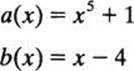
You may check that a(0) = b(0), a(1) = b(l),…, a(4) = b(4); hence a(x) and b(x) are equal functions from ![]() 5 to
5 to ![]() 5. But as polynomials, a(x) and b(x) are quite distinct! (They do not even have the same degree.)
5. But as polynomials, a(x) and b(x) are quite distinct! (They do not even have the same degree.)
It is reassuring to know that this cannot happen when the field F is infinite. Suppose a(x) and b(x) are polynomials over a field F which has infinitely many elements. If a(x) and b(x) are equal as functions, this means that a(c) = b(c) for every c ∈ F. Define the polynomial d(x) to be the difference of a(x) and b(x): d(x) = a(x) − b(x). Then d(c) = 0 for everyc ∈ F. Now, if d(x) were not the zero polynomial, it would be a polynomial (with some finite degree n) having infinitely many roots, and by Theorem 3 this is impossible! Thus, d(x) is the zero polynomial (all its coefficients are equal to zero), and therefore a(x) is the same polynomial as b(x). (They have the same coefficients.)
This tells us that if F is a field with infinitely many elements (such as ![]() ,
, ![]() , or
, or ![]() ), there is no need to distinguish between polynomials and polynomial functions. The difference is, indeed, just a difference of viewpoint.
), there is no need to distinguish between polynomials and polynomial functions. The difference is, indeed, just a difference of viewpoint.
POLYNOMIALS OVER ![]() AND
AND ![]()
In scientific computation a great many functions can be approximated by polynomials, usually polynomials whose coefficients are integers or rational numbers. Such polynomials are therefore of great practical interest. It is easy to find the rational roots of such polynomials, and to determine if a polynomial over ![]() is irreducible over
is irreducible over ![]() . We will do these things next.
. We will do these things next.
First, let us make an important observation:
Let a(x) be a polynomial with rational coefficients, say
![]()
We may now factor out s from all but the first term to get
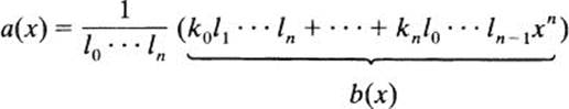
The polynomial b(x) has integer coefficients; and since it differs from a(x) only by a constant factor, it has the same roots as a(x). Thus, for every polynomial with rational coefficients, there is a polynomial with integer coefficients having the same roots. Therefore, for the present we will confine our attention to polynomials with integer coefficients. The next theorem makes it easy to find all the rational roots of such polynomials:
Let s/t be a rational number in simplest form (that is, the integers s and t do not have a common factor greater than 1). Let a(x) = a0 + ⋯ + an xn be a polynomial with integer coefficients.
Theorem 4 If s/t is a root of a(x), then s|a0 and t|an.
PROOF: If s/t is a root of a(x), this means that
a0 + a1(s/t) + ⋯ + an(sn/tn) = 0
Multiplying both sides of this equation by tn we get
a0 tn + a1stn − 1 + ⋯ + ansn = 0 (1)
We may now factor out s from all but the first term to get
− a0tn = s(altn − 1 + ⋯ + ansn − 1
Thus, s /a0tn; and since s and t have no common factors, s|a0. Similarly, in Equation (1), we may factor out t from all but the last term to get
t(a0tn − 1 + ⋯ + an − 1sn − l)= − ansn
Thus, t\ansn; and since s and t have no common factors, t\an. ■
As an example of the way Theorem 4 may be used, let us find the rational roots of a(x) = 2x4 + 7x3 + 5x2 + 7x + 3. Any rational root must be a fraction sit where s is a factor of 3 and t is a factor of 2. The possible roots are therefore ±1, ±3, ±![]() and ±
and ±![]() . Testing each of these numbers by direct substitution into the equation a(x) = 0, we find that −
. Testing each of these numbers by direct substitution into the equation a(x) = 0, we find that − ![]() and − 3 are roots.
and − 3 are roots.
Before going to the next step in our discussion we note a simple but fairly surprising fact.
Lemma Let a(x) = b(x)c(x), where a(x), b(x), and c(x) have integer coefficients. If a prime number p divides every coefficient of a(x), it either divides every coefficient of b(x) or every coefficient of c(x).
PROOF: If this is not the case, let br be the first coefficient of b(x) not divisible by p, and let ct be the first coefficient of c(x) not divisible by p. Now, a(x) = b(x) c(x), so
ar + t = b0cr + t + ⋯ + brct + ⋯ + br + tc0
Each term on the right, except brct is a product biCjwhere either i > r or j > t. By our choice of br and ct, if i > r then p | bi, and j > t then p | cj. Thus, p is a factor of every term on the right with the possible exception of brcn but p is also a factor of ar + t. Thus, p must be a factor of brcn hence of either br or cn and this is impossible. ■
We saw (in the discussion immediately preceding Theorem 4) that any polynomial a{x) with rational coefficients has a constant multiple ka(x), with integer coefficients, which has the same roots as a(x). We can go one better; let a(x)∈ ![]() [x]:
[x]:
Theorem 5 Suppose a(x) can be factored as a(x) = b(x)c(x), where b(x) and c(x) have rational coefficients. Then there are polynomials B(x) and C(x) with integer coefficients, which are constant multiples of b(x) and c(x), respectively, such that a(x) = B(x)C(x).
PROOF. Let k and l be integers such that kb(x) and lc(x) have integer coefficients. Then kla(x) = [kb(x)][lc(x)]. By the lemma, each prime factor of kl may now be canceled with a factor of either kb(x) or lc(x). ■
Remember that a polynomial a(x) of positive degree is said to be reducible over F if there are polynomials b(x) and c(x) in F[x], both of positive degree, such that a(x) = b(x) c(x). If there are no such polynomials, then a(x) is irreducible over F.
If we use this terminology, Theorem 5 states that any polynomial with integer coefficients which is reducible over ![]() is reducible already over
is reducible already over ![]() .
.
In Chapter 25 we saw that every polynomial can be factored into irreducible polynomials. In order to factor a polynomial completely (that is, into irreducibles), we must be able to recognize an irreducible polynomial when we see one! This is not always an easy matter. But there is a method which works remarkably well for recognizing when a polynomial is irreducible over ![]() :
:
Theorem 6: Eisenstein ’ s irreducibility criterion Let
a(x) = a0 + a1x + ⋯ + anxn
be a polynomial with integer coefficients. Suppose there is a prime number p which divides every coefficient of a(x) except the leading cofficient an ; suppose p does not divide an and p2 does not divide a0. Then a(x) is irreducible over![]() .
.
PROOF: If a(x) can be factored over ![]() as a(x) = b(x)c(x), then by Theorem 5 we may assume b(x) and c(x) have integer coefficients: say
as a(x) = b(x)c(x), then by Theorem 5 we may assume b(x) and c(x) have integer coefficients: say
b(x) = b0 + ⋯ + bkxk and c(x) = c0 + ⋯ + cmxm
Now, a0 = b0c0;p divides a0 but p2 does not, so only one of b0, c0 is divisible by p. Say p| c0 and p ∤ b0. Next, an = bkcm and p ∤ an, so p ∤ cm.
Let s be the smallest integer such that p ∤ cs. We have
as = b0cs + b1 cs − 1 + ⋯ + bsc0
and by our choice of cs, every term on the right except b0cs is divisible by p. But as also is divisible by p, and therefore b0cs must be divisible by p. This is impossible because p ∤ b0 and p ∤ cs. Thus, a(x) cannot be factored. ■
For example, x3 + 2x2 + 4x + 2 is irreducible over ![]() because p = 2 satisfies the conditions of Eisenstein’s criterion.
because p = 2 satisfies the conditions of Eisenstein’s criterion.
POLYNOMIALS OVER ![]() AND
AND ![]()
One of the most far-reaching theorems of classical mathematics concerns polynomials with complex coefficients. It is so important in the frame work of traditional algebra that it is called the fundamental theorem of algebra. It states the following:
Every nonconstant polynomial with complex coefficients has a complex root.
(The proof of this theorem is based upon techniques of calculus and can be found in most books on complex analysis. It is omitted here.)
It follows immediately that the irreducible polynomials in ![]() [x] are exactly the polynomials of degree 1. For if a(x) is a polynomial of degree greater than 1 in
[x] are exactly the polynomials of degree 1. For if a(x) is a polynomial of degree greater than 1 in ![]() [x], then by the fundamental theorem of algebra it has a root c and therefore a factor x − c.
[x], then by the fundamental theorem of algebra it has a root c and therefore a factor x − c.
Now, every polynomial in ![]() [x] can be factored into irreducibles. Since the irreducible polynomials are all of degree 1, it follows that if a(x) is a polynomial of degree n over
[x] can be factored into irreducibles. Since the irreducible polynomials are all of degree 1, it follows that if a(x) is a polynomial of degree n over ![]() , it can be factored into
, it can be factored into
a(x) = k(x − c1)(x − c2) ⋯ (x − cn)
In particular, if a(x) has degree n it has n (not necessarily distinct) complex roots c1 … cn.
Since every real number a is a complex number (a = a + 0i), what has just been stated applies equally to polynomials with real coefficients. Specifically, if a(x) is a polynomial of degree n with real coefficients, it can be factored into a(x) = k(x − c1) ⋯ (x − cn), where cl, …,cn are complex numbers (some of which may be real).
For our closing comments, we need the following lemma:
Lemma Suppose a(x) ∈ ![]() [x]. If a + bi is a root of a(x), so is a − bi.
[x]. If a + bi is a root of a(x), so is a − bi.
PROOF: Remember that a − bi is called the conjugate of a + bi. If r is any complex number, we write r for its conjugate. It is easy to see that the function f(r) = ![]() is a homomorphism from
is a homomorphism from ![]() to
to ![]() (in fact, it is an isomorphism). For every real number a, f(a) = a. Thus, if a(x) has real coefficients, then f(a0 + a1r + ⋯ + anrn) = a0 + a1
(in fact, it is an isomorphism). For every real number a, f(a) = a. Thus, if a(x) has real coefficients, then f(a0 + a1r + ⋯ + anrn) = a0 + a1![]() + ⋯ + an
+ ⋯ + an![]() n. Since f(0) = 0, it follows that if r is a root of a(x), so is
n. Since f(0) = 0, it follows that if r is a root of a(x), so is ![]() . ■
. ■
Now let a(x) be any polynomial with real coefficients, and let r = a + bi be a complex root of a(x). Then ![]() is also a root of a(x), so
is also a root of a(x), so
(x − r)(x − ![]() ) = x2 − 2ax + (a2 + b2)
) = x2 − 2ax + (a2 + b2)
and this is a quadratic polynomial with real coefficients! We have thus shown that any polynomial with real coefficients can be factored into polynomials of degree 1 or 1 in ![]() [x]. In particular, the irreducible polynomials of the linear polynomials and [x] are the linear polynomials and the irreducible quadratics (that is, the ax2 + bx + c where b2 − 4ac < 0).
[x]. In particular, the irreducible polynomials of the linear polynomials and [x] are the linear polynomials and the irreducible quadratics (that is, the ax2 + bx + c where b2 − 4ac < 0).
EXERCISES
A. Finding Roots of Polynomials over Finite Fields
In order to find a root of a(x) in a finite field F, the simplest method (if F is small) is to test every element of F by substitution into the equation a(x) = 0.
1 Find all the roots of the following polynomials in ![]() 5[x], and factor the polynomials:
5[x], and factor the polynomials:
x3 + x2 + x + 1; 3x4 + x2 + 1; x5 + 1; x4 + 1; x4 + 4
# 2 Use Fermat’s theorem to find all the roots of the following polynomials in ![]() 7[x]:
7[x]:
x100 − 1; 3x98 + x19 + 3; 2x74 − x55 + 2x + 6
3 Using Fermat ’s theorem, find polynomials of degree ≤6 which determine the same functions as the following polynomials in ![]() 7[x]:
7[x]:
3x75 − 5x54 + 2x13 − x2; 4x10⁸ + 6x101 − 2x81; 3x10³ − x73 + 3x55 − x25
4 Explain why every polynomial in ![]() p[x] has the same roots as a polynomial of degree < p.
p[x] has the same roots as a polynomial of degree < p.
B. Finding Roots of Polynomials over ![]()
# 1 Find all the rational roots of the following polynomials, and factor them into irreducible polynomials in ![]() [x]:
[x]:
![]()
2 Factor each of the preceding polynomials in ![]() [x] and in
[x] and in ![]() [x].
[x].
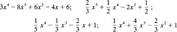
3 Find associates with integer coefficients for each of the following polynomials:
![]()
4 Find all the rational roots of the polynomials in part 3 and factor them over ![]() .
.
5 Does 2x4 + 3x2 − 2 have any rational roots? Can it be factored into two polynomials of lower degree in ![]() [x]? Explain.
[x]? Explain.
C. Short Questions Relating to Roots
Let F be a field.
Prove that parts 1−3 are true in F[x].
1 The remainder of p(x), when divided by x − c, is p(c).
2 (x − c)|(p(x) − p(c)).
3 Every polynomial has the same roots as any of its associates.
4 If a(x) and b(x) have the same roots in F, are they necessarily associates? Explain.
5 Prove: If a(x) is a monic polynomial of degree n, and a(x) has n roots c1, …, cn ∈ F, then a(x) = (x − c1) ⋯ (x − cn).
6 Suppose a(x) and b(x) have degree <n. If a(c) = b(c) for n values of c, prove that a(x) = b(x).
7 There are infinitely many irreducible polynomials in ![]() 5[x].
5[x].
# 8 How many roots does x2 − x have in ![]() 10? In
10? In ![]() 11? Explain the difference.
11? Explain the difference.
D. Irreducible Polynomials in ![]() [x] by Eisenstein’s Criterion (and Variations on the Theme)
[x] by Eisenstein’s Criterion (and Variations on the Theme)
1 Show that each of the following polynomials is irreducible over ![]() :
:
2 It often happens that a polynomial a(y), as it stands, does not satisfy the conditions of Eisenstein’s criterion, but with a simple change of variable y = x + c, it does. It is important to note that if a(x) can be factored into p(x)q(x), then certainly a(x + c) can be factored into p(x + c)q(x + c). Thus, the irreducibility of a(x + c) implies the irreducibility of a(x).
(a) Use the change of variable y = x + l to show that x4 + 4x + l is irreducible in ![]() [x]. [In other words, test (x + l)4 + 4(x + 1) + 1 by Eisenstein’s criterion.]
[x]. [In other words, test (x + l)4 + 4(x + 1) + 1 by Eisenstein’s criterion.]
(b) Find an appropriate change of variable to prove that the following are irreducible in ![]() [x]:
[x]:
x4 + 2x2 − l; x3 −3x + 1; x4 + 1; x4 − 10x2 + 1
# 3 Prove that for any prime p, xp − l + xp − 2 + ⋯ + x + 1 is irreducible in ![]() [x].[HINT: By elementary algebra,
[x].[HINT: By elementary algebra,
(x − 1)(xp −1 + xp − 2 + ⋯ + x + 1) = xp − 1
hence
![]()
Use the change of variable y = x + 1, and expand by the binomial theorem.
4 By Exercise G3 of Chapter 25, the function
h(a0 + a1x + ⋯ + anxn) = an + an − 1x + ⋯ +a0xn
restricted to polynomials with nonzero constant term matches irreducible polynomials with irreducible polynomials. Use this fact to state a dual version of Eisenstein’s irreducibility criterion.
5 Use part 4 to show that each of the following polynomials is irreducible in ![]() [x]:
[x]:
![]()
E. Irreducibility of Polynomials of Degree ≤4
1 Let F be any field. Explain why, if a(x) is a quadratic or cubic polynomial in F[x], a(x) is irreducible in F[x] iff a(x) has no roots in F.
2 Prove that the following polynomials are irreducible in ![]() [x]:
[x]:
![]()
3 Suppose a monic polynomial a(x) of degree 4 in F[x] has no roots in F. Then a(x)is reducible iff it is a product of two quadratics x2 + ax + b and x2 + cx + d, that is, iff
a(x) = x4 + (a + c)x3 + (ac + b + d)x2 + (bc + ad)x +bd
If the coefficients of a(x) cannot be so expressed (in terms of any a, b,c, d ∈ F) then a(x) must be irreducible.
Example a(x) = x4 + 2x3 + x + 1; then bd = 1, so b = d = ±1; thus, bc + ad = ±(a + c), but a + c = 2 and bc + ad = 1; which is impossible.
Prove that the following polynomials are irreducible in ![]() [x] (use Theorem 5, searching only for integer values of a, b, c, d):
[x] (use Theorem 5, searching only for integer values of a, b, c, d):
x4 − 5x2 + 1; 3x4 − x2 − 2; x4 + x3 + 3x + 1
4 Prove that the following polynomials are irreducible in ![]() 5[x]:
5[x]:
2x3 + x2 + 4x + l; x4 + 2; x4 + 4x2 + 2; x4 +1
F. Mapping onto ![]() n to Determine Irreducibility over
n to Determine Irreducibility over ![]()
If h :![]() →
→ ![]() n is the natural homomorphism, let
n is the natural homomorphism, let ![]() :
: ![]() [x] →
[x] → ![]() n[x] be defined by
n[x] be defined by
![]() (a0 + a1x + ⋯ + anxn) = h(a0) + h(al)x + ⋯ + h(an)xn
(a0 + a1x + ⋯ + anxn) = h(a0) + h(al)x + ⋯ + h(an)xn
In Chapter 24, Exercise G, it is proved that ![]() is a homomorphism. Assume this fact and prove:
is a homomorphism. Assume this fact and prove:
# 1 If ![]() (a(x)) is irreducible in
(a(x)) is irreducible in ![]() n[x] and a(x) is monic, then a(x) is irreducible in
n[x] and a(x) is monic, then a(x) is irreducible in ![]() [x].
[x].
2 x4 + 10x3 + 7 is irreducible in ![]() [x] by using the natural homomorphism from
[x] by using the natural homomorphism from ![]() to
to ![]() 5.
5.
3 The following are irreducible in ![]() [x] (find the right value of n and use the natural homomorphism from
[x] (find the right value of n and use the natural homomorphism from ![]() to
to ![]() n):
n):
x4 − 10 x2 + 1; x4 +7 x3 + 14x2 + 3; x5 +1
G. Roots and Factors in A[x] When A Is an Integral Domain
It is a useful fact that Theorems 1, 2, and 3 are still true in A[x] when A is not a field, but merely an integral domain. The proof of Theorem 1 must be altered a bit to avoid using the division algorithm. We proceed as follows:
If a(x) = a0 + a1x + ⋯ + anxn and c is a root of a(x), consider
a(x) − a(c) = a1(x − c) + a2(x2 − c2) + ⋯ + an(xn − cn)
1 Prove that for k = 1, …, n:
ak(xk − ck) = ak(x − c)(xk − l + xk − 2c + ⋯ + ck − l)
2 Conclude from part 1 that a(x) − a(c) = (x − c)q(x) for some q(x).
3 Complete the proof of Theorem 1, explaining why this particular proof is valid when A is an integral domain, not necessarily a field.
4 Check that Theorems 2 and 3 are true in A[x] when A is an integral domain.
H. Polynomial Interpolation
One of the most important applications of polynomials is to problems where we are given several values of x (say, x = a0,a1, …, an) and corresponding values of y (say, y = b0, b,…, bn), and we need to find a function y = f(x) such that f(a0) = b0, f(a1) = b1,…, f(an) = bn. The simplest and most useful kind of function for this purpose is a polynomial function of the lowest possible degree.
We now consider a commonly used technique for constructing a polynomial p(x) of degree n which assumes given values b0, b1,…, bn are given points a0, a1,…,an,. That is,
p(a0)= b0,p(a1)=b, …,p(an) =bn
First, for each i = 0,1, …, n, let
qi(x)= (x − a0) ⋯(x − ai − 1)(x − ai +1) ⋯ (x − an)
1 Show that qi(aj) = 0 for j ≠ i, and qi(ai) ≠ 0.
Let qi(ai) = ci, and define p(x) as follows:
![]()
(This is called the Lagrange interpolation formula.)
2 Explain why p(a0) = b0, p(ax) =,…,p(an)=bn.
# 3 Prove that there is one and only one polynomial p(x) of degree ≤ n such that p(a0) = b0, …, p(an) = bn.
4 Use the Lagrange interpolation formula to prove that if F is a finite field, every function from F to F is equal to a polynomial function. (In fact, the degree of this polynomial is less than the number of elements in F.)
5 If t(x) is any polynomial in F[x], and a0, …, an ∈ F, the unique polynomial p(x) of degree ≤ n such that p(a0) = t(a0), …, p(an) = t(an) is called the Lagrange interpolator for t(x) and a0, …, an. Prove that the remainder, when t(x) is divided by (x − a0)(x − a1) ⋯ (x − an), is the Lagrange interpolator.
I. Polynomial Functions over a Finite Field
1 Find three polynomials in ![]() 5[x] which determine the same function as
5[x] which determine the same function as
x2 − x + 1
2 Prove that xp − x has p roots in ![]() p[x], for any prime p. Draw the conclusion that in
p[x], for any prime p. Draw the conclusion that in ![]() p[x], xp − x can be factored as
p[x], xp − x can be factored as
xp − x = x(x − 1)(x − 2) ⋯ [x − (p − 1)]
3 Prove that if a(x) and b(x) determine the same function in ![]() p[x], then
p[x], then
(xp − x)|(a(x)−b(x))
In the next four parts, let F be any finite field.
# 4 Let a(x) and b(x) be in F[x]. Prove that if a(x) and b(x) determine the same function, and if the number of elements in F exceeds the degree of a(x) as well as the degree of b(x), then a(x) = b(x).
5 Prove: The set of all a(x) which determine the zero function is an ideal of F[x]. What its generator?
6 Let ![]() (F) be the ring of all functions from F to F, defined in the same way as
(F) be the ring of all functions from F to F, defined in the same way as ![]() (
(![]() ). Let h: F[x]→
). Let h: F[x]→ ![]() (F) send every polynomial a(x) to the polynomial function which it determines. Show that h is a homomorphism from F[x] onto
(F) send every polynomial a(x) to the polynomial function which it determines. Show that h is a homomorphism from F[x] onto ![]() (F). (NOTE: To show that h is onto, use Exercise H4.)
(F). (NOTE: To show that h is onto, use Exercise H4.)
7 Let F = {C 1, …, cn} and p(x) = (x − c1) ⋯ (x − cn). Prove that
F[x]/⟨p(x)⟩ ≅ ![]() (F)
(F)