Advanced Calculus of Several Variables (1973)

Part II. Multivariable Differential Calculus

Chapter 3. THE CHAIN RULE

Consider the composition H = G F of two differentiable mappings F : ⁿ → ^m and G : ^m → ^k. For example, might be the price vector of m intermediate products that are manufactured at a factory from nraw materials whose cost vector is x (that is, the components of are the prices of the n raw materials), and H(x) = G(F(x)) the resulting price vector of k final products that are manufactured at a second factory from the mintermediate products. We might wish to estimate the change ΔH_a(h) = H(a + h) − H(a) in the prices of the final products, resulting from a change from a to a + h in the costs of the raw materials. Using the approximations ΔF ≈ dFand ΔG ≈ dG, without initially worrying about the accuracy of our estimates, we obtain

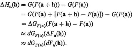
This heuristic “argument” suggests the possibility that the multivariable chain rule takes the form dH_a = dG_F(a) dF_a, analogous to the restatement in Section 1 of the familiar single-variable chain rule.

Theorem 3.1(The Chain Rule) Let U and V be open subsets of ⁿ and ^m respectively. If the mappings F : U → ^m and G : V → ^k are differentiable at and respectively, then their composition H = G Fis differentiable at a, and

In terms of derivatives, we therefore have

In brief, the differential of the composition is the composition of the differentials; the derivative of the composition is the product of the derivatives.

PROOF We must show that

If we define

and

then the fact that F and G are differentiable at a and F(a), respectively, implies that

Then

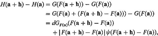
by (Eq. (4) with k = F(a + h) − F(a). Using (3) we then obtain

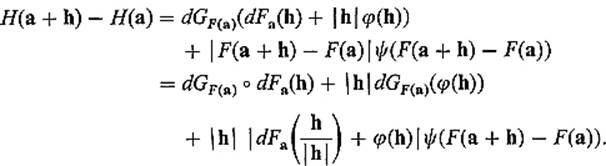
Therefore

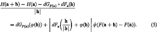
But lim_h→0 dG_F(a)((h)) = 0 because lim_h→0 (h) = 0 and the linear mapping dG_F(a) is continuous. Also lim_h→0 ψ(F(a + h) − F(a)) = 0 because F is continuous at a and lim_k→0 ψ(k) = 0. Finally the number dF_a(h/h) + (h)remains bounded, because and the component functions of the linear mapping dF_a are continuous and therefore bounded on the unit sphere (Theorem I.8.8).

Consequently the limit of (5) is zero as desired. Of course Eq. (2) follows immediately from (1), since the matrix of the composition of two linear mappings is the product of their matrices.

We list in the following examples some typical chain rule formulas obtained by equating components of the matrix equation (2) for various values of n, m, and k. It is the formulation of the chain rule in terms of differential linear mappings which enables us to give a single proof for all of these formulas, despite their wide variety.

Example 1 If n = k = 1, so we have differentiable mappings , then h = g f : → is differentiable with

Here g′(f(t)) is a 1 × m row matrix, and f′(t) is an m × 1 column matrix. In terms of the gradient of g, we have

This is a generalization of the fact that D_vg(a) = g(a) · v ([see Eq. (10) of Section 2]. If we think of f(t) as the position vector of a particle moving in ^m, with g a temperature function on ^m, then 6) gives the rate of change of the temperature of the particle. In particular, we see that this rate of change depends only upon the velocity vector of the particle.

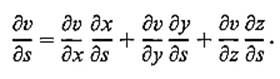
In terms of the component functions f₁, . . . , f_m of f and the partial derivatives of g, (6) becomes

If we write x_i = f_i(t) and u = g(x), following the common practice of using the symbol for a typical value of a function to denote the function itself, then the above equation takes the easily remembered form

Example 2 Given differentiable mappings with composition H : ² → ², the chain rule gives

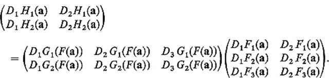
If we write F(s, t) = (x, y, z) and G(x, y, z) = (u, v), this equation can be rewritten

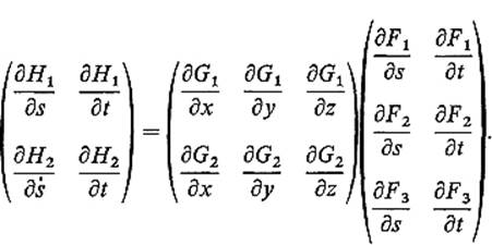
For example, we have

Writing

to go all the way with variables representing functions, we obtain formulas such as

and

The obvious nature of the formal pattern of chain rule formulas expressed in terms of variables, as above, often compensates for their disadvantage of not containing explicit reference to the points at which the various derivatives are evaluated.

Example 3 Let T : ² → ² be the familiar “polar coordinate mapping” defined by T(r, θ) = (r cos θ, r sin θ) (Fig. 2.10). Given a differentiable function f : ² → , define g = f T, so g(r, θ) = f(r cos θ, r sin θ). Then the chain rule gives

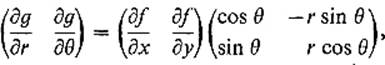
so

Thus we have expressed the partial derivatives of g in terms of those of f, that is, in terms of ∂f/∂x = D₁f(r cos θ, r sin θ) and ∂f/∂y = D₂f(r cos θ, r sin θ).

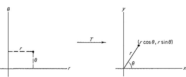
Figure 2.10

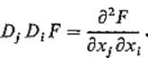
The same can be done for the second order partial derivatives. Given a differentiable mapping F : ⁿ → ^m, the partial derivative D_iF is again a mapping from ⁿ to ^m. If it is differentiable at a, we can consider the second partial derivative

The classical notation is

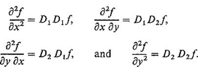
For example, the function f : ² → has second-order partial derivatives

Continuing Example 3 we have

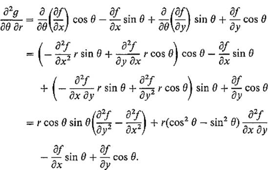
In the last step we have used the fact that the “mixed partial derivatives” ∂²f/∂x ∂y and ∂²f/∂y ∂x are equal, which will be established at the end of this section under the hypothesis that they are continuous.

In Exercise 3.9, the student will continue in this manner to show that Laplace's equation

transforms to

in polar coordinates.

As a standard application of this fact, consider a uniform circular disk of radius 1, whose boundary is heated in such a way that its temperature on the boundary is given by the function g : [0, 2π] → , that is,

for each ; see Fig. 2.11. Then certain physical considerations suggest that the temperature function u(r, θ) on the disk satisfies Laplace's equation (8) in polar coordinates. Now it is easily verified directly (do this) that, for each positive integer n, the functions rⁿ cos nθ and rⁿ sin nθ satisfy Eq. (8). Therefore, if a Fourier series expansion

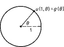
Figure 2.11

for the function g can be found, then the series

is a plausible candidate for the temperature function u(r, θ)—it reduces to g(θ) when r = 1, and satisfies Eq. (8), if it converges for all and if its first and second order derivatives can be computed by termwise differentiation.

Example 4 Consider an infinitely long vibrating string whose equilibrium position lies along the x-axis, and denote by f(x, t) the displacement of the point x at time t (Fig. 2.12). Then physical considerations suggest that f satisfies the one-dimensional wave equation

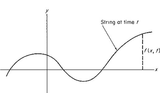
Figure 2.12

where a is a certain constant. In order to solve this partial differential equation, we make the substitution

where A, B, C, D are constants to be determined. Writing g(u, v) = f(Au + Bv, Cu + Dv), we find that

(see Exercise 3.7). If we choose , C = 1/2a, D = −1/2a, then it follows from this equation and (9) that

This implies that there exist functions , ψ : → such that

In terms of x and t, this means that

Suppose now that we are given the initial position

and the initial velocity D₂f(x, 0) = G(x) of the string. Then from (10) we obtain

and

so

by the fundamental theorem of calculus. We then solve (11) and (12) for (x) and ψ(x):

Upon substituting x + at for x in (13), and x − at for x in (14), and adding, we obtain

This is “ d‘Alembert’s solution ” of the wave equation. If G(x) ≡ 0, the picture looks like Fig. 2.13. Thus we have two “waves” moving in opposite directions.

The last two examples illustrate the use of chain rule formulas to “transform” partial differential equations so as to render them more amenable to solution.

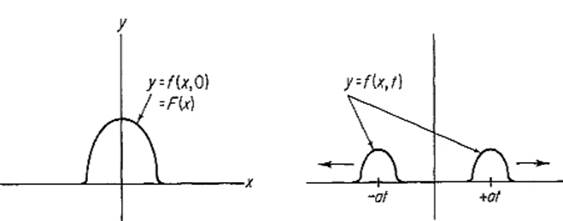
Figure 2.13

We shall now apply the chain rule to generalize some of the basic results of single-variable calculus. First consider the fact that a function defined on an open interval is constant if and only if its derivative is zero there. Since the function f(x, y) defined for x ≠ 0 by

has zero derivative (or gradient) where it is defined, it is clear that some restriction must be placed on the domain of definition of a mapping if we are to generalize this result correctly.

The open set is said to be connected if and only if given any two points a and b of U, there is a differentiable mapping : → U such that (0) = a and (1) = b (Fig. 2.14). Of course the mapping F : U → ^m is said to be constant on U if F(a) = F(b) for any two points , so that there exists such that F(x) = c for all .

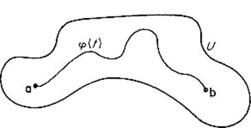
Figure 2.14

Theorem 3.2 Let U be a connected open subset of ⁿ. Then the differentiable mapping F : U → ^m is constant on U if and only if F′(x) = 0 (that is, the zero matrix) for all .

PROOF Since F is constant if and only if each of its component functions is, and the matrix F′(x) is zero if and only if each of its rows is, we may assume that F is real valued, F = f : U → . Since we already know that f′(x) = 0 if fis constant, suppose that f′(x) = f(x) = 0 for all .

Given a and , let : → U be a differentiable mapping with (0) = a, (1) = b.

If g = f : → , then

for all , by Eq. (6) above. Therefore g is constant on [0, 1], so

Corollary 3.3 Let F and G be two differentiable mappings of the connected set into ^m. If F′(x) = G′(x) for all , then there exists such that

for all . That is, F and G differ only by a constant.

PROOF Apply Theorem 3.2 to the mapping F − G.

Now consider a differentiable function f : U → , where U is a connected open set in ². We say that f is independent of y if there exists a function g : → such that f(x, y) = g(x) if . At first glance it might seem that f is independent of y if D₂ f = 0 on U. To see that this is not so, however, consider the function f defined on

by f(x, y) = x² if x > 0 or y > 0, and f(x, y) = −x² if and y< 0. Then D₂f(x, y) = 0 on U. But f(−1, 1) = 1, while f(−1, −1) = −1. We leave it as an exercise for the student to formulate a condition on U under which D₂f = 0 doesimply that f is independent of y.

Let us recall here the statement of the mean value theorem of elementary single-variable calculus. If f : [a, b] → is a differentiable function, then there exists a point such that

The mean value theorem generalizes to real-valued functions on ⁿ (however it is in general false for vector-valued functions—see Exercise 1.12. In the following statement of the mean value theorem in ⁿ, by the line segmentfrom a to b is meant the set of all points in ⁿ of the form (1 − t)a + tb for .

Theorem 3.4 (Mean Value Theorem) Suppose that U is an open set in ⁿ, and that a and b are two points of U such that U contains the line segment L from a to b. If f is a differentiable real-valued function on U, then

for some point .

PROOF Let be the mapping of [0, 1] onto L defined by

Then is differentiable with ′(t) = b − a. Hence the composition g = f is differentiable by the chain rule. Since g : [0, 1] → , the single-variable mean value theorem gives a point such that g(1) − g(0) = g′(ξ). If , we then have

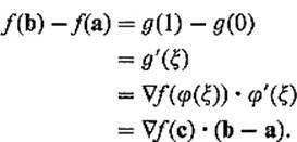
Note that here we have employed the chain rule to deduce the mean value theorem for functions of several variables from the single-variable mean value theorem.

Next we are going to use the mean value theorem to prove that the second partial derivatives D_j D_if and D_j D_if are equal under appropriate conditions. First note that, if we write b = a + h in the mean value theorem, then its conclusion becomes

for some .

Recall the notation Δf_a(h) = f(a + h) − f(a). The mapping Δf_a: ⁿ → is sometimes called the “first difference” of f at a. The “second difference” of f at a is a function of two points h, k defined by (see Fig. 2.15)

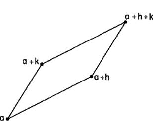
Figure 2.15

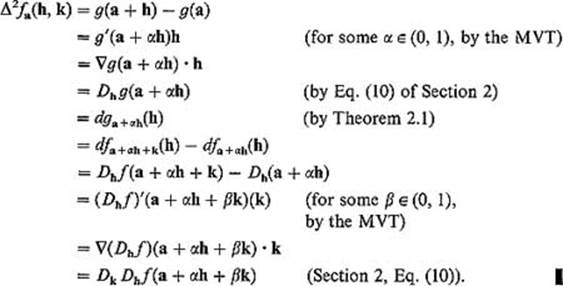
The desired equality of second order partial derivatives will follow easily from the following lemma, which expresses in terms of the second order directional derivative D_k D_hf(x), which is by definition the derivative with respect to k of the function D_hf at x, that is

Lemma 3.5 Let U be an open set in ⁿ which contains the parallelogram determined by the points a, a + h, a + k, a + h + k. If the real-valued function f and its directional derivative D_hf are both differentiable on U, then there exist numbers such that

PROOF Define g(x) in a neighborhood of the line segment from a to a + h by

Then g is differentiable, with

and

Theorem 3.6 Let f be a real-valued function defined on the open set U in ⁿ. If the first and second partial derivatives of f exist and are continuous on U, then D_i D_jf = D_j D_if on U.

PROOF Theorem 2.5 implies that both f and its partial derivatives D₁ f and D₂ f are differentiable on U. We can therefore apply Lemma 3.5 with h = he_i and k = ke_j, provided that h and k are sufficiently small that U contains the rectangle with vertices a, a + he_i, a + ke_j, a + he_i + ke_j. We obtain such that

If we apply Lemma 3.5 again with h and k interchanged, we obtain α₂, such that

But it is clear from the definition of Δ²f_a that

so we conclude that

using the facts that .

If we now divide the previous equation by hk, and take the limit as h → 0, k → 0, we obtain

because both are continuous at a.

REMARK In this proof we actually used only the facts that f, D₁f, D₂f are differentiable on U, and that D_j D_i f and D_i D_j f are continuous at the point a. Exercise 3.16 shows that the continuity of D_j D_if and D_i D_j f at a are necessary for their equality there.

Exercises

3.1Let f : be differentiable at each point of the unit circle x² + y² = 1. Show that, if u is the unit tangent vector to the circle which points in the counterclockwise direction, then

3.2If f and g are differentiable real-valued functions on , show that

(a) (f + g) = f + g,

(b) (fg) = fg + g f,

(c) (fⁿ) = nfⁿ⁻¹ f.

3.3Let F, G : be differentiable mappings, and h : a differentiable function. Given , show that

(a) D_u(F + G) = D_u F + D_u G,

(b) D_u+v F = D_u F + D_v F,

(c) D_u(hF) = (D_u h)F + h(D_u F).

3.4Show that each of the following two functions is a solution of the heat equation (k a constant).

(a)

(b)

3.5Suppose that f : has continuous second order partial derivatives. Set x = s + t, y = s − t to obtain g : defined by g(s, t) = f(s + t, s − t). Show that

that is, that

3.6Show that

if we set x = 2s + t, y = s − t. First state what this actually means, in terms of functions.

3.7If g(u, v) = f(Au + Bv, Cu + Dv), where A, B, C, D are constants, show that

3.8Let f : be a function with continuous second partial derivatives, so that ∂²f/∂x ∂y = ∂²f/∂y ∂x. If g : is defined by g(r, θ) = f(r cos θ, r sin θ), show that

This gives the length of the gradient vector in polar coordinates.

3.9If f and g are as in the previous problem, show that

This gives the 2-dimensional Laplacian in polar coordinates.

3.10Given a function f: with continuous second partial derivatives, define

where ρ, θ, ϕ are the usual spherical coordinates. We want to express the 3-dimensional Laplacian

in spherical coordinates, that is, in terms of partial derivatives of F.

(a)First define g(r, θ, z) = f(r cos θ, r sin θ, z) and conclude from Exercise 3.9 that

(b)Now define F(ρ, θ, ϕ) = g(ρ sin ϕ, θ, ρ cos ϕ). Noting that, except for a change in notation, this is the same transformation as before, deduce that

3.11(a)If if show that

for x ≠ 0.

(b)Deduce from (a) that, if ²f = 0, then

where a and b are constants.

3.12Verify that the functions rⁿ cos nθ and rⁿ sin nθ satisfy the 2-dimensional Laplace equation in polar coordinates.

3.13If f(x, y, z) = (1/r) g(t − r/c), where c is constant and r = (x² + y² + z²)^1/2, show that f satisfies the 3-dimensional wave equation

3.14The following example illustrates the hazards of denoting functions by real variables. Let w = f(x, y, z) and z = g(x, y). Then

since ∂x/∂x = 1 and ∂y/∂x = 0. Hence ∂w/∂z ∂z/∂x = 0. But if w = x + y + z and z = x + y, then ∂w/∂z = ∂z/∂x = 1, so we have 1 = 0. Where is the mistake?

3.15Use the mean value theorem to show that 5.18 < [(4.1)² + (3.2)²]^1/2 < 5.21. Hint: Note first that (5)² < x² + y² < (5.5)² if 4 < x < 4.1 and 3 < y < 3.2.

3.16Define f : by f(x, y) = xy(x² − y²)/(x² + y²) unless x = y = 0, and f(0, 0) = 0.

(a)Show that D₁ f(0, y) = −y and D₂f(x, 0) = x for all x and y.

(b)Conclude that D₁D₂ f(0, 0) and D₂ D₁ f(0, 0) exist but are not equal.

3.17The object of this problem is to show that, by an appropriate transformation of variables, the general homogeneous second order partial differential equation

with constant coefficients can be reduced to either Laplace's equation, the wave equation, or the heat equation.

(a)If ac − b² > 0, show that the substitution s = (bx − ay)/(ac − b²)^1/2, t = y changes (*) to

(b)If ac − b² = 0, show that the substitution s = bx − ay, t = y changes (*) to

(c)If ac − b² < 0, show that the substitution

changes (*) to ∂²u/∂s ∂t = 0.

3.18Let F : ^m be differentiable at . Given a differentiable curve φ: with φ(0) = a, φ′(0) = v, define ψ = F φ, and show that ψ′(0) = dF_a(v). Hence, if : is a second curve with (0) = a, ′(0) = v, and = F, then ′(0) = ψ′(0), because both are equal to dF_a(v). Consequently F maps curves through a, with the same velocity vector, to curves through F(a) with the same velocity vector.

3.19Let φ: , f: ^m, and g : be differentiable mappings. If h = g fφ show that h′(t) = g(f(φ(t))) • D_φ′(t)f(φ(t)).