Advanced Calculus of Several Variables (1973)
Part II. Multivariable Differential Calculus
Chapter 5. MAXIMA AND MINIMA, MANIFOLDS, AND LAGRANGE MULTIPLIERS
In this section we generalize the Lagrange multiplier method to ![]() n. Let D be a compact (that is, by Theorem I.8.6, closed and bounded) subset of
n. Let D be a compact (that is, by Theorem I.8.6, closed and bounded) subset of ![]() n. If the function f : D
n. If the function f : D ![]() is continuous then, by Theorem I.8.8, there exists a point
is continuous then, by Theorem I.8.8, there exists a point ![]() at which f attains its (absolute) maximum value on D (and similarly f attains an absolute minimum value at some point of D). The point p may be either a boundary point or an interior point of D. Recall that p is a boundary point of D if and only if every open ball centered at p contains both points of D and points of
at which f attains its (absolute) maximum value on D (and similarly f attains an absolute minimum value at some point of D). The point p may be either a boundary point or an interior point of D. Recall that p is a boundary point of D if and only if every open ball centered at p contains both points of D and points of ![]() n − D; an interior point of D is a point of D that is not a boundary point. Thus p is an interior point of D if and only if Dcontains some open ball centered at p. The set of all boundary (interior) points of D is called its boundary (interior).
n − D; an interior point of D is a point of D that is not a boundary point. Thus p is an interior point of D if and only if Dcontains some open ball centered at p. The set of all boundary (interior) points of D is called its boundary (interior).
For example, the open ball Br(p) is the interior of the closed ball ![]() r(p); the sphere Sr(p) =
r(p); the sphere Sr(p) = ![]() r(p) − Br(p) is its boundary.
r(p) − Br(p) is its boundary.
We say that the function f : D ![]() has a local maximum (respectively, local minimum) on D at the point
has a local maximum (respectively, local minimum) on D at the point ![]() if and only if there exists an open ball B centered at p such that
if and only if there exists an open ball B centered at p such that ![]() [respectively,
[respectively, ![]() for all points
for all points ![]() . Thus f has a local maximum on D at the point p if its value at p is at least as large as at any “nearby” point of D.
. Thus f has a local maximum on D at the point p if its value at p is at least as large as at any “nearby” point of D.
In applied maximum–minimum problems the set D is frequently the set of points on or within some closed and bounded (n − 1)-dimensional surface S in ![]() n; S is then the boundary of D. We will see in Corollary 5.2 that, if the differentiable function f : D
n; S is then the boundary of D. We will see in Corollary 5.2 that, if the differentiable function f : D ![]() has a local maximum or minimum at the interior point
has a local maximum or minimum at the interior point ![]() , then p must be a critical point of f, that is, a point at which all of the 1st partial derivatives of f vanish, so
, then p must be a critical point of f, that is, a point at which all of the 1st partial derivatives of f vanish, so ![]() f(p) = 0. The critical points of f can (in principle) be found by “setting the partial derivatives of f all equal to zero and solving for the coordinates x1, . . . , xn.” The location of critical points in higher dimensions does not differ essentially from their location in 2-dimensional problems of the sort discussed at the end of the previous section.
f(p) = 0. The critical points of f can (in principle) be found by “setting the partial derivatives of f all equal to zero and solving for the coordinates x1, . . . , xn.” The location of critical points in higher dimensions does not differ essentially from their location in 2-dimensional problems of the sort discussed at the end of the previous section.
If, however, p is a boundary point of D at which f has a local maximum or minimum on D, then the situation is quite different—the location of such points is a Lagrange multiplier type of problem; this section is devoted to such problems. Our methods will be based on the following result (see Fig. 2.23).
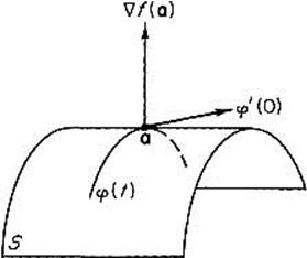
Figure 2.23
Theorem 5.1 Let S be a set in ![]() n, and φ :
n, and φ : ![]() S a differentiable curve with φ(0) = a. If f is a differentiable real-valued function defined on some open set containing S, and f has a local maximum (or local minimum) on S at a,then the gradient vector
S a differentiable curve with φ(0) = a. If f is a differentiable real-valued function defined on some open set containing S, and f has a local maximum (or local minimum) on S at a,then the gradient vector ![]() f(a) is orthogonal to the velocity vector φ′(0).
f(a) is orthogonal to the velocity vector φ′(0).
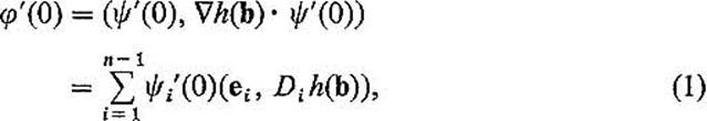
PROOF The composite function h = f ![]() φ :
φ : ![]() is differentiable at
is differentiable at ![]() , and attains a local maximum (or local minimum) there. Therefore h′(0) = 0, so the chain rule gives
, and attains a local maximum (or local minimum) there. Therefore h′(0) = 0, so the chain rule gives
It is an immediate corollary that interior local maximum–minimum points are critical points.
Corollary 5.2 If U is an open subset of ![]() n, and a
n, and a![]() is a point at which the differentiable function f : U →
is a point at which the differentiable function f : U → ![]() has a local maximum or local minimum, then a is a critical point of f. That is,
has a local maximum or local minimum, then a is a critical point of f. That is, ![]() f(a) = 0.
f(a) = 0.
PROOF Given ![]() , define φ :
, define φ : ![]() by φ(t) = a + tv, so φ′(t) ≡ v. Then Theorem 5.1 gives
by φ(t) = a + tv, so φ′(t) ≡ v. Then Theorem 5.1 gives
![]()
Since ![]() f(a) is thus orthogonal to every vector
f(a) is thus orthogonal to every vector ![]() , it follows that
, it follows that ![]() f(a) = 0.
f(a) = 0.
![]()
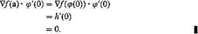
Example 1 Suppose we want to find the maximum and minimum values of the function f(x, y, z) = x + y + z on the unit sphere
![]()
in ![]() 3. Theorem 5.1 tells us that, if a = (x, y, z) is a point at which f attains its maximum or minimum on S2, then
3. Theorem 5.1 tells us that, if a = (x, y, z) is a point at which f attains its maximum or minimum on S2, then ![]() f(a) is orthogonal to every curve on S2 passing through a, and is therefore orthogonal to the sphere at a (that is, to its tangent plane at a). But it is clear that a itself is orthogonal to S2 at a. Hence
f(a) is orthogonal to every curve on S2 passing through a, and is therefore orthogonal to the sphere at a (that is, to its tangent plane at a). But it is clear that a itself is orthogonal to S2 at a. Hence ![]() f(a) and a ≠ 0 are collinear vectors (Fig. 2.24), so
f(a) and a ≠ 0 are collinear vectors (Fig. 2.24), so ![]() f(a) = λa for some number λ. But
f(a) = λa for some number λ. But ![]() f = (1, 1, 1), so
f = (1, 1, 1), so
![]()
so x = y = z = 1/λ. Since x2 + y2 + z2 = 1, the two possibilities are a = ![]() Since Theorem I.8.8 implies that f does attain maximum and minimum values on S2, we conclude that these are
Since Theorem I.8.8 implies that f does attain maximum and minimum values on S2, we conclude that these are ![]()
![]() , respectively.
, respectively.
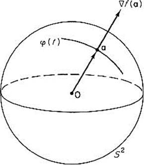
Figure 2.24
The reason we were able to solve this problem so easily is that, at every point, the unit sphere S2 in ![]() 3 has a 2-dimensional tangent plane which can bedescribed readily in terms of its normal vector. We want to generalize (and systematize) the method of Example 1, so as to be able to find the maximum and minimum values of a differentiable real-valued function on an (n − 1)-dimensional surface in
3 has a 2-dimensional tangent plane which can bedescribed readily in terms of its normal vector. We want to generalize (and systematize) the method of Example 1, so as to be able to find the maximum and minimum values of a differentiable real-valued function on an (n − 1)-dimensional surface in ![]() n.
n.
We now need to make precise our idea of what an (n − 1)-dimensional surface is. To start with, we want an (n − 1)-dimensional surface (called an (n − 1)-manifold in the definition below) to be a set in ![]() n which has at each point an (n − 1)-dimensional tangent plane. The set M in
n which has at each point an (n − 1)-dimensional tangent plane. The set M in ![]() n is said to have a k-dimensional tangent plane at the point
n is said to have a k-dimensional tangent plane at the point ![]() if the union of all tangent lines at a, to differentiable curves on M passing through a, is a k-dimensional plane (that is, is a translate of a k-dimensional subspace of
if the union of all tangent lines at a, to differentiable curves on M passing through a, is a k-dimensional plane (that is, is a translate of a k-dimensional subspace of ![]() n). see Fig. 2.25.
n). see Fig. 2.25.
A manifold will be defined as a union of sets called “patches.” Let πi: ![]() n−1 denote the projection mapping which simply deletes the ith coordinate, that is,
n−1 denote the projection mapping which simply deletes the ith coordinate, that is,
![]()
Figure 2.25
where the symbol ![]() i means that the coordinate xi has been deleted from the n-tuple, leaving an (n − 1)-tuple, or point of
i means that the coordinate xi has been deleted from the n-tuple, leaving an (n − 1)-tuple, or point of ![]() n−1. The set P in
n−1. The set P in ![]() n is called an (n − 1)-dimensional patch if and only if for some positive integer
n is called an (n − 1)-dimensional patch if and only if for some positive integer ![]() , there exists a differentiable function h : U
, there exists a differentiable function h : U ![]() , on an open subset
, on an open subset ![]() , such that
, such that
![]()
In other words, P is the graph in ![]() n of the differentiable function h, regarding h as defined on an open subset of the (n − 1)-dimensional coordinate plane πi(
n of the differentiable function h, regarding h as defined on an open subset of the (n − 1)-dimensional coordinate plane πi(![]() n) that is spanned by the unit basis vectors e1, . . . , ei−1, ei+1, . . . , en (see Fig. 2.26). To put it still another way, the ith coordinate of a point of P is a differentiable function of its remaining n − 1 coordinates. We will see in the proof of Theorem 5.3 that every (n − 1)-dimensional patch in
n) that is spanned by the unit basis vectors e1, . . . , ei−1, ei+1, . . . , en (see Fig. 2.26). To put it still another way, the ith coordinate of a point of P is a differentiable function of its remaining n − 1 coordinates. We will see in the proof of Theorem 5.3 that every (n − 1)-dimensional patch in ![]() n has an (n − 1)-dimensional tangent plane at each of its points.
n has an (n − 1)-dimensional tangent plane at each of its points.
The set M in ![]() n is called an (n − 1)-dimensional manifold, or simply an
n is called an (n − 1)-dimensional manifold, or simply an
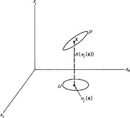
Figure 2.26
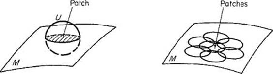
Figure 2.27
(n − 1)-manifold, if and only if each point ![]() lies in an open subset U of
lies in an open subset U of ![]() n such that
n such that ![]() is an (n − 1)-dimensional patch (see Fig. 2.27). Roughly speaking, a manifold is simply a union of patches, although this is not quite right, because in an arbitrary union of patches two of them might intersect “wrong.”
is an (n − 1)-dimensional patch (see Fig. 2.27). Roughly speaking, a manifold is simply a union of patches, although this is not quite right, because in an arbitrary union of patches two of them might intersect “wrong.”
Example 2 The unit circle x2 + y2 = 1 is a 1-manifold in ![]() 2, since it is the union of the 1-dimensional patches corresponding to the open semicircles x > 0, x < 0, y > 0, y < 0 (see Fig. 2.28). Similarly the unit sphere x2 + y2 + z2 = 1 is a 2-manifold in
2, since it is the union of the 1-dimensional patches corresponding to the open semicircles x > 0, x < 0, y > 0, y < 0 (see Fig. 2.28). Similarly the unit sphere x2 + y2 + z2 = 1 is a 2-manifold in ![]() 3, since it is covered by six 2-dimensional patches —the upper and lower, front and back, right and left open hemispheres determined by z > 0, z < 0, x > 0, x < 0, y > 0, y < 0, respectively. The student should be able to generalize this approach so as to see that the unit sphere Sn−1 in
3, since it is covered by six 2-dimensional patches —the upper and lower, front and back, right and left open hemispheres determined by z > 0, z < 0, x > 0, x < 0, y > 0, y < 0, respectively. The student should be able to generalize this approach so as to see that the unit sphere Sn−1 in ![]() n is an (n − 1)-manifold.
n is an (n − 1)-manifold.
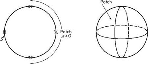
Figure 2.28
Example 3 The “torus” T in ![]() 3, obtained by rotating about the z-axis the circle (y − 1)2 + z2 = 4 in the yz-plane, is a 2-manifold (Fig. 2.29). The upper and lower open halves of T, determined by the conditions z > 0 and z < 0 respectively, are 2-dimensional patches; each is clearly the graph of a differentiable function defined on the open “annulus” 1 < x2 + y2 < 9 in the xy-plane. These two patches cover all of T except for the points on the circles x2 + y2= 1 and x2 + y2 = 9 in the xy-plane. Additional patches in T, covering these two circles,
3, obtained by rotating about the z-axis the circle (y − 1)2 + z2 = 4 in the yz-plane, is a 2-manifold (Fig. 2.29). The upper and lower open halves of T, determined by the conditions z > 0 and z < 0 respectively, are 2-dimensional patches; each is clearly the graph of a differentiable function defined on the open “annulus” 1 < x2 + y2 < 9 in the xy-plane. These two patches cover all of T except for the points on the circles x2 + y2= 1 and x2 + y2 = 9 in the xy-plane. Additional patches in T, covering these two circles,
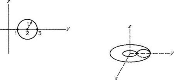
Figure 2.29
must be defined in order to complete the proof that T is a 2-manifold (see Exercise 5.1).
The following theorem gives the particular property of (n − 1)-manifolds in ![]() n which is important for maximum–minimum problems.
n which is important for maximum–minimum problems.
Theorem 5.3 If M is an (n − 1)-dimensional manifold in ![]() n, then, at each of its points, M has an (n − 1)-dimensional tangent plane.
n, then, at each of its points, M has an (n − 1)-dimensional tangent plane.
PROOF Given ![]() , we want to show that the union of all tangent lines at a, to differentiable curves through a on M, is an (n − 1)-dimensional plane or, equivalently, that the set of all velocity vectors of such curves is an (n − 1)-dimensional subspace of
, we want to show that the union of all tangent lines at a, to differentiable curves through a on M, is an (n − 1)-dimensional plane or, equivalently, that the set of all velocity vectors of such curves is an (n − 1)-dimensional subspace of ![]() n.
n.
The fact that M is an (n − 1)-manifold means that, near a, M coincides with the graph of some differentiable function h : ![]() . That is, for some
. That is, for some ![]() for all points (x1, . . . , xn) of M sufficiently close to a. Let us consider the case i = n (from which the other cases differ only by a permutation of the coordinates).
for all points (x1, . . . , xn) of M sufficiently close to a. Let us consider the case i = n (from which the other cases differ only by a permutation of the coordinates).
Let φ : ![]() → M be a differentiable curve with φ(0) = a, and define ψ :
→ M be a differentiable curve with φ(0) = a, and define ψ : ![]() n−1 by ψ = π
n−1 by ψ = π ![]() φ, where π :
φ, where π : ![]() n−1 is the usual projection. If
n−1 is the usual projection. If ![]()
![]() , then the image of φ near a lies directly “above” the image of ψnear b. That is, φ(t) = (ψ(t), h(ψ(t)) for t sufficiently close to 0. Applying the chain rule, we therefore obtain
, then the image of φ near a lies directly “above” the image of ψnear b. That is, φ(t) = (ψ(t), h(ψ(t)) for t sufficiently close to 0. Applying the chain rule, we therefore obtain
where e1, . . . , en−1 are the unit basis vectors in ![]() n−1. Consequently φ′(0) lies in the (n − 1)-dimensional subspace of
n−1. Consequently φ′(0) lies in the (n − 1)-dimensional subspace of ![]() n spanned by the n − 1 (clearly linearly independent) vectors
n spanned by the n − 1 (clearly linearly independent) vectors
![]()
Conversely, given a vector ![]() of this (n − 1)-dimensional space, consider the differentiable curve φ :
of this (n − 1)-dimensional space, consider the differentiable curve φ : ![]() → M defined by
→ M defined by
![]()
where ![]() . It is then clear from (1) that φ′(0) = v. Thus every point of our (n − 1)-dimensional subspace is the velocity vector of some curve through a on M.
. It is then clear from (1) that φ′(0) = v. Thus every point of our (n − 1)-dimensional subspace is the velocity vector of some curve through a on M.
![]()
In order to apply Theorem 5.3, we need to be able to recognize an (n − 1)-manifold (as such) when we see one. We give in Theorem 5.4 below a useful sufficient condition that a set ![]() be an (n − 1)-manifold. For its proof we need the following basic theorem, which will be established in Chapter III. It asserts that if g :
be an (n − 1)-manifold. For its proof we need the following basic theorem, which will be established in Chapter III. It asserts that if g : ![]() is a continuously differentiable function, and g(a) = 0 with some partial derivative Dig(a) ≠ 0, then near a the equation
is a continuously differentiable function, and g(a) = 0 with some partial derivative Dig(a) ≠ 0, then near a the equation
g(x1,.....,xn) = 0
can be “solved for xi as a function of the remaining variables.” This implies that, near a, the set S = g−1(0) looks like an (n − 1)-dimensional patch, hence like an (n − 1)-manifold (see Fig. 2.30). We state this theorem with i = n.
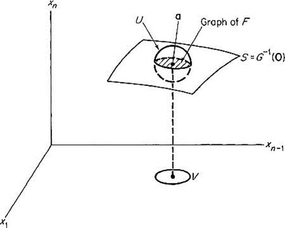
Figure 2.30
Implicit Function Theorem Let G : ![]() be continuously differentiable, and suppose that G(a) = 0 while Dn G(a) ≠ 0. Then there exists a neighborhood U of a and a differentiable function F defined on a neighborhood V of
be continuously differentiable, and suppose that G(a) = 0 while Dn G(a) ≠ 0. Then there exists a neighborhood U of a and a differentiable function F defined on a neighborhood V of ![]() , such that
, such that
![]()
In particular,
![]()
for all![]() .
.
Theorem 5.4 Suppose that g : ![]() is continuously differentiable. If M is the set of all those points
is continuously differentiable. If M is the set of all those points ![]() at which
at which ![]() g(x) ≠ 0, then M is an (n − 1)-manifold. Given
g(x) ≠ 0, then M is an (n − 1)-manifold. Given ![]() , the gradient vector
, the gradient vector ![]() g(a) is orthogonal to the tangent plane to M at a.
g(a) is orthogonal to the tangent plane to M at a.
PROOF Let a be a point of M, so g(a) = 0 and ![]() g(a) ≠ 0. Then Dig(a) = 0 for some
g(a) ≠ 0. Then Dig(a) = 0 for some ![]() . Define G :
. Define G : ![]() by
by
![]()
Then G(b) = 0 and Dn G(b) ≠ 0, where b = (a1, . . . , ai−1, . . . , ai+1, . . . , an, ai). Let ![]() be the open sets, and F : V
be the open sets, and F : V ![]() the implicitly defined function, supplied by the implicit function theorem, so that
the implicitly defined function, supplied by the implicit function theorem, so that
![]()
Now let W be the set of all points ![]() such that
such that ![]() . Then
. Then ![]() is clearly an (n − 1)-dimensional patch; in particular,
is clearly an (n − 1)-dimensional patch; in particular,
![]()
To prove that ![]() g(a) is orthogonal to the tangent plane to M at a, we need to show that, if φ :
g(a) is orthogonal to the tangent plane to M at a, we need to show that, if φ : ![]() M is a differentiable curve with φ(0) = a, then the vectors
M is a differentiable curve with φ(0) = a, then the vectors ![]() g(a) and φ′(0) are orthogonal. But the composite function g
g(a) and φ′(0) are orthogonal. But the composite function g ![]() φ :
φ : ![]() is identically zero, so the chain rule gives
is identically zero, so the chain rule gives
![]()
For example, if g(x) = x12 + · · · + xn2 − 1, then M is the unit sphere Sn−1 in ![]() n, so Theorem 5.4 provides a quick proof that Sn−1 is an (n − 1)-manifold.
n, so Theorem 5.4 provides a quick proof that Sn−1 is an (n − 1)-manifold.
We are finally ready to “put it all together.”
Theorem 5.5 Suppose g : ![]() is continuously differentiable, and let M be the set of all those points
is continuously differentiable, and let M be the set of all those points ![]() at which both g(x) = 0 and
at which both g(x) = 0 and ![]() g(x) ≠ 0. If the differentiable function f :
g(x) ≠ 0. If the differentiable function f : ![]() attains a local maximum or minimum on M at the point
attains a local maximum or minimum on M at the point ![]() , then
, then
![]()
for some number λ (called the “Lagrange multiplier”).
PROOF By Theorem 5.4, M is an (n − 1)-manifold, so M has an (n − 1)-dimensional tangent plane by Theorem 5.3. The vectors ![]() f(a) and
f(a) and ![]() g(a) are both orthogonal to this tangent plane, by Theorems 5.1 and 5.4, respectively. Since the orthogonal complement to an (n − 1)-dimensional subspace of
g(a) are both orthogonal to this tangent plane, by Theorems 5.1 and 5.4, respectively. Since the orthogonal complement to an (n − 1)-dimensional subspace of ![]() n is 1-dimensional, by Theorem I.3.4, it follows that
n is 1-dimensional, by Theorem I.3.4, it follows that ![]() f(a) and
f(a) and ![]() g(a) are collinear. Since
g(a) are collinear. Since ![]() g(a) ≠ 0, this implies that
g(a) ≠ 0, this implies that ![]() f(a) is a multiple of
f(a) is a multiple of ![]() g(a).
g(a).
![]()
According to this theorem, in order to maximize or minimize the function f : ![]() subject to the “constraint equation”
subject to the “constraint equation”
![]()
it suffices to solve the n + 1 scalar equations
![]()
for the n + 1 “unknowns” x1, . . . , xn, λ. If these equations have several solutions, we can determine which (if any) gives a maximum and which gives a minimum by computing the value of f at each. This in brief is the“ Lagrange multiplier method.”
Example 4 Let us reconsider Example 5 of Section 4. We want to find the rectangular box of volume 1000 which has the least total surface area A. If
![]()
our problem is to minimize the function f on the 2-manifold in ![]() 3 given by g(x, y, z) = 0. Since
3 given by g(x, y, z) = 0. Since ![]() f = (2y + 2z, 2x + 2z, 2x + 2y) and
f = (2y + 2z, 2x + 2z, 2x + 2y) and ![]() g = (yz, xz, xy), we want to solve the equations
g = (yz, xz, xy), we want to solve the equations
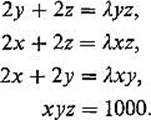
Upon multiplying the first three equations by x, y, and z respectively, and then substituting xyz = 1000 on the right hand sides, we obtain
![]()
from which it follows easily that x = y = z. Since xyz = 1000, our solution gives a cube of edge 10.
Now we want to generalize the Lagrange multiplier method so as to be able to maximize or minimize a function f : ![]() subject to several constraint equations
subject to several constraint equations
![]()
where m < n. For example, suppose that we wish to maximize the function f(x, y, z) = x2 + y2 + z2 subject to the conditions x2 + y2 = 1 and x + y + z = 0. The intersection of the cylinder x2 + y2 = 1 and the plane x + y + z = 0 is an ellipse in ![]() 3, and we are simply asking for the maximum distance (squared) from the origin to a point of this ellipse.
3, and we are simply asking for the maximum distance (squared) from the origin to a point of this ellipse.
If G : ![]() m is the mapping whose component functions are the functions g1, . . . , gm, then equations (3) may be rewritten as G(x) = 0. Experience suggests that the set S = G−1(0) may (in some sense) be an (n − m)-dimensional surface in
m is the mapping whose component functions are the functions g1, . . . , gm, then equations (3) may be rewritten as G(x) = 0. Experience suggests that the set S = G−1(0) may (in some sense) be an (n − m)-dimensional surface in ![]() n. To make this precise, we need to define k-manifolds in
n. To make this precise, we need to define k-manifolds in ![]() n, for all k < n.
n, for all k < n.
Our definition of (n − 1)-dimensional patches can be rephrased to say that ![]() is an (n − 1)-dimensional patch if and only if there exists a permutation x1, . . . , xn of the coordinates x1, . . . , xn in
is an (n − 1)-dimensional patch if and only if there exists a permutation x1, . . . , xn of the coordinates x1, . . . , xn in ![]() n, and a differentiable function h : U
n, and a differentiable function h : U ![]() on an open set
on an open set ![]() , such that
, such that
![]()
Similarly we say that the set ![]() is a k-dimensional patch if and only if there exists a permutation xin of x1, . . . , xn, and a differentiable mapping h : U →
is a k-dimensional patch if and only if there exists a permutation xin of x1, . . . , xn, and a differentiable mapping h : U → ![]() n−k defined on an open set
n−k defined on an open set ![]() , such that,
, such that,
![]()
Thus P is simply the graph of h, regarded as a function of xik, rather than x1, . . . , xk as usual; the coordinates xik+1, . . . , xinof a point of P are differentiable functions of its remaining k coordinates (see Fig. 2.31).
The set ![]() is called a k-dimensional manifold in
is called a k-dimensional manifold in ![]() n, or k-manifold, if every point of M lies in an open subset V of
n, or k-manifold, if every point of M lies in an open subset V of ![]() n such that
n such that ![]() is a k-dimensional patch. Thus a k-manifold is a set which is made up of k-dimensional
is a k-dimensional patch. Thus a k-manifold is a set which is made up of k-dimensional
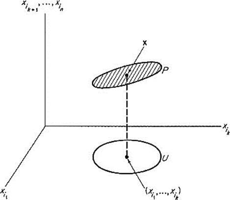
Figure 2.31
patches, in the same way that an (n − 1)-manifold is made up of (n − 1)-dimensional patches. For example, it is easily verified that the circle x2 + y2 = 1 in the xy-plane is a 1-manifold in ![]() 3. This is a special case of the fact that, if M is a k-manifold in
3. This is a special case of the fact that, if M is a k-manifold in ![]() n, and
n, and ![]() n is regarded as a subspace of
n is regarded as a subspace of ![]() p (p > n), then M is a k-manifold in
p (p > n), then M is a k-manifold in ![]() p (Exercise 5.2).
p (Exercise 5.2).
In regard to both its statement and its proof (see Exercise 5.16), the following result is the expected generalization of Theorem 5.3.
Theorem 5.6 If M is a k-dimensional manifold in ![]() n then, at each of its points, M has a k-dimensional tangent plane.
n then, at each of its points, M has a k-dimensional tangent plane.
In order to generalize Theorem 5.4, the following generalization of the implicit function theorem is required; its proof will be given in Chapter III.
Implicit Mapping Theorem Let G : ![]() m (m < n) be a continuously differentiable mapping. Suppose that G(a) = 0 and that the rank of the derivative matrix G′(a) is m. Then there exists a permutation xi1,....,xin of the coordinates in
m (m < n) be a continuously differentiable mapping. Suppose that G(a) = 0 and that the rank of the derivative matrix G′(a) is m. Then there exists a permutation xi1,....,xin of the coordinates in ![]() n, an open subset U of
n, an open subset U of ![]() n containing a, an open subset V of
n containing a, an open subset V of ![]() n − m containing
n − m containing ![]() , and a differentiable mapping h : V
, and a differentiable mapping h : V ![]() m such that each point X
m such that each point X![]() lies on S = G−1(0) if and only if
lies on S = G−1(0) if and only if ![]() and
and
![]()
Recall that the m × n matrix G′(a) has rank m if and only if its m row vectors ![]() G1(a), . . . ,
G1(a), . . . , ![]() Gm(a) (the gradient vectors of the component functions of G) are linearly independent (Section I.5). If m = 1, so G = g :
Gm(a) (the gradient vectors of the component functions of G) are linearly independent (Section I.5). If m = 1, so G = g : ![]() , this is just the condition that
, this is just the condition that ![]() g(a) ≠ 0, so some partial derivative Dig(a) ≠ 0. Thus the implicit mapping theorem is indeed a generalization of the implicit function theorem.
g(a) ≠ 0, so some partial derivative Dig(a) ≠ 0. Thus the implicit mapping theorem is indeed a generalization of the implicit function theorem.
The conclusion of the implicit mapping theorem asserts that, near a, the m equations
![]()
can be solved (uniquely) for the m variables ![]() as differentiable functions of the variables
as differentiable functions of the variables ![]() . Thus the set S = G−1(0) looks, near a, like an (n − m)-dimensional manifold. Using the implicit mapping theorem in place of the implicit function theorem, the proof of Theorem 5.4 translates into a proof of the following generalization.
. Thus the set S = G−1(0) looks, near a, like an (n − m)-dimensional manifold. Using the implicit mapping theorem in place of the implicit function theorem, the proof of Theorem 5.4 translates into a proof of the following generalization.
Theorem 5.7 Suppose that the mapping G : ![]() m is continuously differentiable. If M is the set of all those points
m is continuously differentiable. If M is the set of all those points ![]() for which the rank of G′(x) is m, then M is an (n − m)-manifold. Given
for which the rank of G′(x) is m, then M is an (n − m)-manifold. Given ![]() , the gradient vectors
, the gradient vectors ![]() G1(a), . . . ,
G1(a), . . . , ![]() Gm(a), of the component functions of G, are all orthogonal to the tangent plane to M at a (see Fig. 2.32).
Gm(a), of the component functions of G, are all orthogonal to the tangent plane to M at a (see Fig. 2.32).
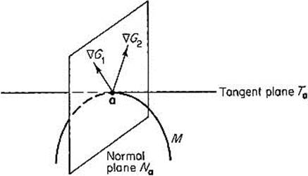
Figure 2.32
In brief, this theorem asserts that the solution set of m equations in n > m variables is, in general, an (n − m)-dimensional manifold in ![]() n. Here the phrase “in general” means that, if our equations are
n. Here the phrase “in general” means that, if our equations are
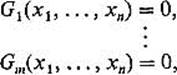
we must know that the functions G1, . . . , Gm are continuously differentiable, and also that the gradient vectors ![]() G1, . . . ,
G1, . . . , ![]() Gm are linearly independent at each point of M = G−1(0), and finally that M is nonempty to start with.
Gm are linearly independent at each point of M = G−1(0), and finally that M is nonempty to start with.
Example 5 If G : ![]() 2 is defined by
2 is defined by
![]()
then G−1(0) is the intersection M of the unit sphere x2 + y2 + z2 = 1 and the plane x + y + z = 1. Of course it is obvious that M is a circle. However, to conclude from Theorem 5.7 that M is a 1-manifold, we must first verify that ![]() G1= (2x, 2y, 2z) and
G1= (2x, 2y, 2z) and ![]() G2 = (1, 1, 1) are linearly independent (that is, not collinear) at each point of M. But the only points of the unit sphere, where
G2 = (1, 1, 1) are linearly independent (that is, not collinear) at each point of M. But the only points of the unit sphere, where ![]() G1 is collinear with (1, 1, 1), are
G1 is collinear with (1, 1, 1), are ![]() and
and ![]() ,
,![]() neither of which lies on the plane x + y + z = 1.
neither of which lies on the plane x + y + z = 1.
Example 6 If G : ![]() 4 →
4 → ![]() 2 is defined by
2 is defined by
![]()
the gradient vectors
![]()
are linearly independent at each point of M = G−1(0) (Why?), so M is a 2-manifold in ![]() 4 (it is a torus).
4 (it is a torus).
Example 7 If g(x, y, z) = x2 + y2 − z2, then S = g−1(0) is a double cone which fails to be a 2-manifold only at the origin. Note that (0, 0, 0) is the only point of S where ![]() g = (2x, 2y, − 2z) is zero.
g = (2x, 2y, − 2z) is zero.
We are finally ready for the general version of the Lagrange multiplier method.
Theorem 5.8 Suppose G : ![]() m (m < n) is continuously differentiable, and denote by M the set of all those points
m (m < n) is continuously differentiable, and denote by M the set of all those points ![]() such that G(x) = 0, and also the gradient vectors
such that G(x) = 0, and also the gradient vectors ![]() G1(x), . . . ,
G1(x), . . . , ![]() Gm(x) are linearly independent. If the differentiable function f :
Gm(x) are linearly independent. If the differentiable function f : ![]() attains a local maximum or minimum on M at the point
attains a local maximum or minimum on M at the point ![]() , then there exist real numbers λ1, . . . , λm (called Lagrange multipliers) such that
, then there exist real numbers λ1, . . . , λm (called Lagrange multipliers) such that
![]()
PROOF By Theorem 5.7, M is an (n − m)-manifold, and therefore has an (n − m)-dimensional tangent plane Ta at a, by Theorem 5.6. If Na is the orthogonal complement to the translate of Ta to the origin, then Theorem I.3.4 implies that dim Na = m. The linearly independent vectors ![]() G1(a), . . . ,
G1(a), . . . , ![]() Gm(a) lie in Na (Theorem 5.7), and therefore constitute a basis for Na. Since, by Theorem 5.1,
Gm(a) lie in Na (Theorem 5.7), and therefore constitute a basis for Na. Since, by Theorem 5.1, ![]() f(a) also lies in Na, it follows that
f(a) also lies in Na, it follows that ![]() f(a) is a linear combination of the vectors
f(a) is a linear combination of the vectors ![]() G1(a), . . . ,
G1(a), . . . , ![]() Gm(a).
Gm(a).
![]()
In short, in order to locate all points ![]() at which f can attain a maximum or minimum value, it suffices to solve the n + m scalar equations
at which f can attain a maximum or minimum value, it suffices to solve the n + m scalar equations
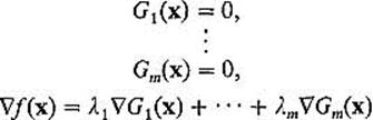
for the n + m “unknowns” x1, . . . , xn, λ1, . . . , λm.
Example 8 Suppose we want to maximize the function f(x, y, z) = x on the circle of intersection of the plane z = 1 and the sphere x2 + y2 + z2 = 4 (Fig. 2.33). We define g : ![]() 2 by g1(x, y, z) = z − 1 and g2(x, y, z) = x2 + y2 + z2 − 1. Then g−1(0) is the given circle of intersection.
2 by g1(x, y, z) = z − 1 and g2(x, y, z) = x2 + y2 + z2 − 1. Then g−1(0) is the given circle of intersection.
Since ![]() f = (1, 0, 0),
f = (1, 0, 0), ![]() g1 = (0, 0, 1),
g1 = (0, 0, 1), ![]() g2 = (2x, 2y, 2z), we want to solve the equations
g2 = (2x, 2y, 2z), we want to solve the equations
![]()
We obtain the two solutions ![]() for (x, y, z), so the maximum is
for (x, y, z), so the maximum is ![]() and the minimum is
and the minimum is ![]() .
.
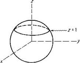
Figure 2.33
Example 9 Suppose we want to find the minimum distance between the circle x2 + y2 = 1 and the line x + y = 4 (Fig. 2.34). Given a point (x, y) on the circle and a point (u, v) in the line, the square of the distance between them is
![]()
So we want to minimize f subject to the “constraints” x2 + y2 = 1 and u + v = 4. That is, we want to minimize the function f : ![]() 4 →
4 → ![]() on the 2-manifold M in
on the 2-manifold M in ![]() 4 defined by the equations
4 defined by the equations
![]()
and
![]()
Note that the gradient vectors ![]() g1 = (2x, 2y, 0, 0) and
g1 = (2x, 2y, 0, 0) and ![]() g2 = (0, 0, 1, 1) are never collinear, so Theorem 5.7 implies that M = g−1(0) is a 2-manifold. Since
g2 = (0, 0, 1, 1) are never collinear, so Theorem 5.7 implies that M = g−1(0) is a 2-manifold. Since
![]()
Theorem 5.8 directs us to solve the equations
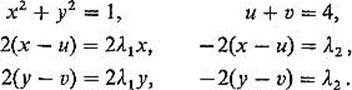
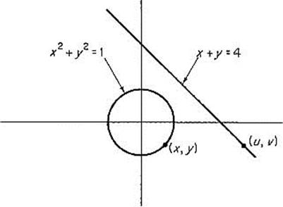
Figure 2.34
From −2(x − u) = λ2 = − 2(y − v), we see that
x – u = y – v
If λ1 were 0, we would have (x, y) = (u, v) from 2(x − u) = 2λ1x and 2(y − v) = 2λ1y. But the circle and the line have no point in common, so we conclude that λ1 ≠ 0. Therefore
![]()
so finally u = v. Substituting x = y and u = v into x2 + y2 = 1 and u + v = 4, we obtain ![]() . Consequently, the closest points on the circle and line are
. Consequently, the closest points on the circle and line are ![]() and (2, 2).
and (2, 2).
Example 10 Let us generalize the preceding example. Suppose M and N are two manifolds in ![]() n, defined by g(x) = 0 and h(x) = 0, where
n, defined by g(x) = 0 and h(x) = 0, where
![]()
are mappings satisfying the hypotheses of Theorem 5.7. Let p![]() M and q
M and q![]() N be two points which are closer together than any other pair of points of M and N.
N be two points which are closer together than any other pair of points of M and N.
If x = (x1, . . . , xn) and y = (y1, . . . , yn) are any two points of M and N respectively, the square of the distance between them is
![]()
So to find the points p and q, we need to minimize the function f : ![]() 2n →
2n → ![]() on the manifold in
on the manifold in ![]() 2n =
2n = ![]() n ×
n × ![]() n defined by the equation G(x, y) = 0, where
n defined by the equation G(x, y) = 0, where
![]()
That is, G : ![]() 2n
2n ![]() m+k is defined by
m+k is defined by
![]()
Theorem 5.8 implies that ![]() f = λ1
f = λ1![]() G1 + · · · + λm+k
G1 + · · · + λm+k ![]() Gm+k at (p, q). Since
Gm+k at (p, q). Since
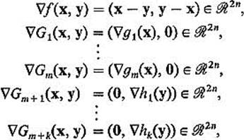
we conclude that the solution satisfies
![]()
Since (p, q) is assumed to be the solution, we conclude that the line joining p and q is both orthogonal to M at p and orthogonal to N at q.
Let us apply this fact to find the points on the unit sphere x2 + y2 + z2 = 1 and the plane u + v + w = 3 which are closest. The vector (x, y, z) is orthogonal to the sphere at (x, y, z), and (1, 1, 1) is orthogonal to the plane at (u, v, w). So the vector (x − u, y − v, z − w) from (x, y, z) to (u, v w) must be a multiple of both (x, y, z) and (1, 1, 1):
![]()
Hence x = y = z and u = v = w. Consequently the points ![]() and (1, 1, 1) are the closest points on the sphere and plane, respectively.
and (1, 1, 1) are the closest points on the sphere and plane, respectively.
Exercises
5.1Complete the proof that the torus in Example 3 is a 2-manifold.
5.2If M is a k-manifold in ![]() n, and
n, and ![]() , show that M is a k-manifold in
, show that M is a k-manifold in ![]() p.
p.
5.3If M is a k-manifold in ![]() m and N is an l-manifold in
m and N is an l-manifold in ![]() n, show that M × N is a (k + l)-manifold in
n, show that M × N is a (k + l)-manifold in ![]() m+n =
m+n = ![]() m ×
m × ![]() n.
n.
5.4Find the points of the ellipse x2/9 + y2/4 = 1 which are closest to and farthest from the point (1, 1).
5.5Find the maximal volume of a closed rectangular box whose total surface area is 54.
5.6Find the dimensions of a box of maximal volume which can be inscribed in the ellipsoid
![]()
5.7Let the manifold S in ![]() n be defined by g(x) = 0. If p is a point not on S, and q is the point of S which is closest to p, show that the line from p to q is perpendicular to S at q. Hint: Minimize f(x) =
n be defined by g(x) = 0. If p is a point not on S, and q is the point of S which is closest to p, show that the line from p to q is perpendicular to S at q. Hint: Minimize f(x) = ![]() x − p
x − p![]() 2 on S.
2 on S.
5.8Show that the maximum value of the function f(x) = x12x22 · · · xn2 on the sphere ![]() That is
That is ![]() .
.
Given n positive numbers a1, . . . , an, define
![]()
Then x12 + · · · + xn2 = 1, so
![]()
Thus the geometric mean of n positive numbers is no greater than their arithmetic mean.
5.9Find the minimum value of f(x) = n−1(x1 + · · · + xn) on the surface g(x) = x1x2 · · · xn − 1 = 0. Deduce again the geometric–arithmetic means inequality.
5.10The planes x + 2y + z = 4 and 3x + y + 2z = 3 intersect in a straight line L. Find the point of L which is closest to the origin.
5.11Find the highest and lowest points on the ellipse of intersection of the cylinder x2 + y2 = 1 and the plane x + y + z = 1.
5.12Find the points of the line x + y = 10 and the ellipse x2 + 2y2 = 1 which are closest.
5.13Find the points of the circle x2 + y2 = 1 and the parabola y2 = 2(4 − x) which are closest.
5.14Find the points of the ellipsoid x2 + 2y2 + 3z2 = 1 which are closest to and farthest from the plane x + y + z = 10.
5.15Generalize the proof of Theorem 5.3 so as to prove Theorem 5.6.
5.16Verify the last assertion of Theorem 5.7.