Advanced Calculus of Several Variables (1973)
Part II. Multivariable Differential Calculus
Chapter 6. TAYLOR'S FORMULA FOR SINGLE-VARIABLE FUNCTIONS
In order to generalize the results of Section 4, and in particular to apply the Lagrange multiplier method to classify critical points for functions of n variables, we will need Taylor‘s formula for functions on ![]() n. As preparation for the treatment in Section 7 of the multivariable Taylor’s formula, this section is devoted to the single-variable Taylor's formula.
n. As preparation for the treatment in Section 7 of the multivariable Taylor’s formula, this section is devoted to the single-variable Taylor's formula.
Taylor's formula provides polynomial approximations to general functions. We will give examples to illustrate both the practical utility and the theoretical applications of such approximations.
If f: ![]() is differentiable at a, and R(h) is defined by
is differentiable at a, and R(h) is defined by
![]()
then it follows immediately from the definition of f′(a) that
![]()
With x = a + h, (1) and (2) become
![]()
where
![]()
The linear function P(x − a) = f(a) + f′(a)(x − a) is simply that first degree polynomial in (x − a) whose value and first derivative at a agree with those of f at a. The kth degree polynomial in (x − a), such that the values of it and of its first k derivatives at a agree with those of f and its first k derivatives f′, f′, f(3), . . . , f(k) at a, is
![]()
This fact may be easily checked by repeated differentiation of Pk(x − a). The polynomial Pk(x − a) is called the kth degree Taylor polynomial of f at a.
The remainder f(x) − Pk(x − a) is denoted by Rk(x − a), so
![]()
With x − a = h, this becomes
![]()
where
![]()
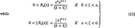
In order to make effective use of Taylor polynomials, we need an explicit formula for Rk(x − a) which will provide information as to how closely Pk(x − a) approximates f(x) near a. For example, whenever we can show that
![]()
this will mean that f is arbitrarily closely approximated by its Taylor polynomials; they can then be used to calculate f(x) as closely as desired. Equation (4), or (4′), together with such an explicit expression for the remainder Rk, is referred to as Taylor's formula. The formula for Rk given in Theorem 6.1 below is known as the Lagrange form of the remainder.
Theorem 6.1 Suppose that the (k + 1)th derivative f(k+1) of f: ![]() exists at each point of the closed interval I with endpoints a and x. Then there exists a point ζ between a and x such that
exists at each point of the closed interval I with endpoints a and x. Then there exists a point ζ between a and x such that
![]()
Hence
![]()
or
![]()
with h = x − a.
REMARK This is a generalization of the mean value theorem; in particular, P0(x − a) = f(a), so the case k = 0 of the theorem is simply the mean value theorem
![]()
for the function f on the interval I. Moreover the proof which we shall give for Taylor's formula is a direct generalization of the proof of the mean value theorem. So for motivation we review the proof of the mean value theorem (slightly rephrased).
First we define R0(t) for ![]() (for convenience we assume h > 0) by
(for convenience we assume h > 0) by
![]()
and note that
![]()
while
![]()
Then we define φ: [0, h] ![]() by
by
![]()
where the constant K is chosen so that Rolle's theorem [the familiar fact that, if f is a differentiable function on [a, b] with f(a) = f(b) = 0, then there exists a point ![]() will apply to φ on [0, h], that is,
will apply to φ on [0, h], that is,
![]()
so it follows that φ(h) = 0. Hence Rolle's theorem gives a ![]() such that
such that
![]()
Hence K = f′(ζ) where ζ = a + ![]() , so from (9) we obtain R0(h) = f′(ζ)h as desired.
, so from (9) we obtain R0(h) = f′(ζ)h as desired.
PROOF OF THEOREM 6.1 We generalize the above proof, labeling the formulas with the same numbers (primed) to facilitate comparison.
First we define Rk(t) for ![]() by
by
![]()
and note that
![]()
while
![]()
The reason for (6′) is that the first k derivatives of Pk(x − a) at a, and hence the first k derivatives of Pk(t) at 0, agree with those of f at a, while (7′) follows from the fact that ![]() because Pk(t) is a polynomial of degree k.
because Pk(t) is a polynomial of degree k.
Now we define φ: [0, h] ![]() by
by
![]()
where the constant K is chosen so that Rolle's theorem will apply to φ on [0, h], that is,
![]()
so it follows that φ(h) = 0. Hence Rolle's theorem gives a point ![]() such that φ′(
such that φ′(![]() 1) = 0.
1) = 0.
It follows from (6′) and (7′) that

while
![]()
Therefore we can apply Rolle's theorem to φ′ on the interval [0, ![]() 1] to obtain a point
1] to obtain a point ![]() such that φ′(
such that φ′(![]() 2) = 0.
2) = 0.
![]()
By (10), φ′ satisfies the hypotheses of Rolle‘s theorem on [0, ![]() 2], so we can continue in this way. After k + 1 applications of Rolle’s theorem, we finally obtain a point
2], so we can continue in this way. After k + 1 applications of Rolle’s theorem, we finally obtain a point ![]() such that φ(k+1)(tk+1) = 0. From the second equation in (10) we then obtain
such that φ(k+1)(tk+1) = 0. From the second equation in (10) we then obtain
![]()
with ζ = a + ![]() k+1. Finally (9′) gives
k+1. Finally (9′) gives
![]()
as desired.
![]()
Corollary 6.2 If, in addition to the hypotheses of Theorem 6.1, ![]()
![]()
It follows that
![]()
In particular, (12) holds if f(k+1) is continuous at a, because it will then necessarily be bounded (by some M) on some open interval containing a.
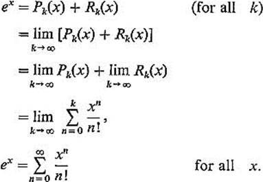
Example 1 As a standard first example, we take f(x) = ex, a = 0. Then f(k)(x) = ex, so f(k)(0) = 1 for all k. Then
![]()
and
![]()
for some ζ between 0 and x. Therefore
In either case the elementary fact that
![]()
implies that limk→∞ Rk(x) = 0 for all x, so
[To verify the elementary fact used above, choose a fixed integer m such that ![]() . If k > m, then
. If k > m, then
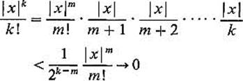
as k → ∞.]
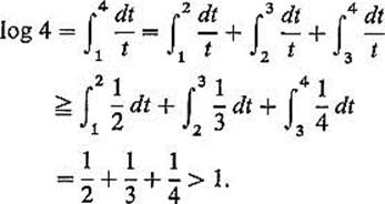
In order to calculate the value of ex with preassigned accuracy by simply calculating Pk(x), we must be able to estimate the error Rk(x). For this we need the preliminary estimate e < 4. Since log e = 1 and log x is a strictly increasing function, to verify that e < 4 it suffices to show that log 4 > 1. But
From (see 13) we now see that Rk(x) < 4/(k + 1)! if ![]() this can be used to compute e to any desired accuracy (Exercise 6.1).
this can be used to compute e to any desired accuracy (Exercise 6.1).
Example 2 To calculate ![]() , and consider the first degree Taylor formula
, and consider the first degree Taylor formula
![]()
![]() .
.
Since ![]()
![]()
so we conclude that
![]()
(actually ![]() to five places).
to five places).
The next two examples give a good indication of the wide range of application of Taylor's formula.
Example 3 We show that the number e is irrational. To the contrary, suppose that e = p/q where p and q are positive integers. Since e = 2.718 to three decimal places (see Exercise 6.1), it is clear that e is not an integral multiple of 1, ![]() , By Example 1, we can write
, By Example 1, we can write
![]()
where
![]()
since 0 < ζ < 1 and e < 3. Upon multiplication of both sides of the above equation by q!, we obtain
![]()
But this is a contradiction, because the left-hand side (q − 1)! p is an integer, but the right-hand side is not, because
![]()
since q > 3.
Example 4 We use Taylor's formula to prove that, if f′ − f = 0 on R and f(0) = f′(0) = 0, then f = 0 on ![]() .
.
Since f′ = f, we see by repeated differentiation that f(k) exists for all k; in particular,
![]()
Since f(0) = f′(0) = 0, it follows that f(k)(0) = 0 for all k. Consequently Theorem 4.1 gives, for each k, a point ![]() such that
such that
![]()
Since there are really only two different derivatives involved, and each is continuous because it is differentiable, there exists a constant M such that
![]()
Hence ![]() so we conclude that f(x) = 0.
so we conclude that f(x) = 0.
Now we apply Taylor's formula to give sufficient conditions for local maxima and minima of real-valued single-variable functions.
Theorem 6.3 Suppose that f(k+1) exists in a neighborhood of a and is continuous at a. Suppose also that
![]()
but f(k)(a) ≠ 0. Then
(a)f has a local minimum at a if k is even, and f(k)(a) > 0;
(b)f has a local maximum at a if k is even and f(k)(a) < 0;
(c)f has neither a maximum nor a minimum at a if k is odd.
This is a generalization of the familiar “second derivative test” which asserts that, if f′(a) = 0, then f has a local minimum at a if f′(a) > 0, and a local maximum at a if f′(a) < 0. The three cases can be remembered by thinking of the three graphs in Fig. 2.35.
If f(k)(a) = 0 for all k, then Theorem 6.3 provides no information as to the behavior of f in a neighborhood of a. For instance, if
![]()
then it turns out that f(k)(0) = 0 for all k, so Theorem 6.3 does not apply. However it is obvious that f has a local minimum at 0, since f(x) > 0 for x ≠ 0 (Fig. 2.36).
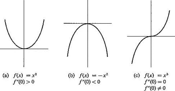
Figure 2.35
As motivation for the proof of Theorem 6.3, let us consider first the “second-derivative test.” If f′(a) = 0, then Taylor's formula with k = 2 is
![]()
where limx→a R2(x − a)/(x − a)2 = 0 by Corollary 6.2 (assuming that f(3) is continuous at a). By transposing f(a) and dividing by (x − a)2, we obtain
![]()
so it follows that
![]()
If f′(a) > 0, this implies that f(x) − f(a) > 0 if x is sufficiently close to a, since (x − a)2 > 0 for all x ≠ a. Thus f(a) is a local minimum. Similarly f(a) is a local maximum if f′(a) < 0.
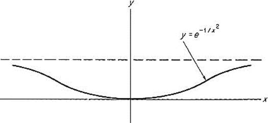
Figure 2.36
In similar fashion we can show that, if f′(a) = f′(a) = 0 while f(3)(a) ≠ 0, then f has neither a maximum nor a minimum at a (this fact might be called the “third-derivative test”). To see this, we look at Taylor's formula with k = 3,
![]()
where limx→a R3(x − a)/(x − a)3 = 0. Transposing f(a) and then dividing by (x − a)3, we obtain
![]()
so it follows that
![]()
If, for instance, f(3)(a) > 0, we see that [f(x) − f(a)]/(x − a)3 > 0 if x is sufficiently close to a. Since (x − a)3 > 0 if x > a and (x − a)3 < 0 if x < a, it follows that, for x sufficiently close to a, f(x) − f(a) < 0 if x < a, and f(x) − f(a) < 0 if x < a. These inequalities are reversed if f(3)(a) < 0. Consequently f(a) is neither a local maximum nor a local minimum.
The proof of Theorem 6.3 simply consists of replacing 2 and 3 in the above discussion by k, the order of the first nonzero derivative of f at the critical point a. If k is even the argument is the same as when k = 2, while if k is odd it is the same as when k = 3.
PROOF OF THEOREM 6.3 Because of the hypotheses, Taylor's formula takes the form
![]()
where limx→a Rk(x − a)/(x − a)k = 0 by Corollary 6.2. If we transpose f(a), divide by (x − a)k, and then take limits as x → a, we therefore obtain
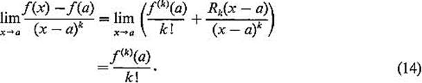
In case (a), limx→a[f(x) − f(a)]/(x − a)k > 0 by (14), so it follows that there exists a Δ > 0 such that
![]()
Since k is even in this case, (x − a)k > 0 whether x > a or x < a, so
![]()
Therefore f(a) is a local minimum.
The proof in case (b) is the same except for reversal of the inequalities.
In case (c), supposing f(k)(a) > 0, there exists (just as above) a Δ > 0 such that
![]()
But now, since k is odd, the sign of (x − a)k depends upon whether x < a or x > a. The same is then true of f(x) − f(a), so f(x) < f(a) if x > a, and f(x) > f(a) if x > a; the situation is reversed if f(k)(a) < 0. In either event it is clear that f(a) is neither a local maximum nor a local minimum.
![]()
Let us look at the case k = 2 of Theorem 6.3 in a bit more detail. We have
![]()
where limx→a R2(x − a)/(x − a)2 = 0. Therefore, given ![]() , there exists a Δ > 0 such that
, there exists a Δ > 0 such that
![]()
which implies that
![]()
Substituting (16) into (15), we obtain
![]()
If f′(a) > 0, then ![]() are both positive because
are both positive because ![]() . It follows that the graphs of the equations
. It follows that the graphs of the equations
![]()
are then parabolas opening upwards with vertex (a, f(a)) (see Fig. 2.37). The fact that inequality (17) holds if 0 < ![]() x − a
x − a![]() < Δ means that the part of the graph of y = f(x), over the interval (a − Δ, a + Δ), lies between these two parabolas. This makes it clear that f has a local minimum at a if f′(a) > 0.
< Δ means that the part of the graph of y = f(x), over the interval (a − Δ, a + Δ), lies between these two parabolas. This makes it clear that f has a local minimum at a if f′(a) > 0.
The situation is similar if f′(a) < 0, except that the parabolas open downward, so f has a local maximum at a.
In the case k = 3, these parabolas are replaced by the cubic curves
![]()
which look like Fig. 2.35c above, so f has neither a maximum nor a minimum at a.
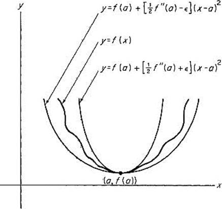
Figure 2.37
Exercises
6.1Show that e = 2.718, accurate to three decimal places. Hint: Refer to the error estimate at the end of Example 1; choose k such that 4/(k + 1)! < 10−4.
6.2Prove that, if we compute ex by the approximation
![]()
then the error will not exceed 0.001 if ![]() . Then compute
. Then compute ![]() accurate to two decimal places.
accurate to two decimal places.
6.3If ![]() .Conclude that
.Conclude that
![]()
is the only kth degree polynomial in (x − a) such that the values of it and its first k derivatives at a agree with those of f at a.
6.4(a) Show that the values of the sine function for angles between 40° and 50° can be computed by means of the approximation
![]()
with 4-place accuracy. Hint: With f(x) = sin x, a = π/4, k = 3, show that the error is less than 10−5, since 5° = π/36 < 1/10 rad.
(b) Compute sin 50°, accurate to four decimal places.
6.5Show that
![]()
for all x.
6.6Show that the kth degree Taylor polynomial of f(x) = log x at a = 1 is
![]()
and that limk→∞ Rk(x − 1) = 0 if x![]() (1,2). Then compute
(1,2). Then compute ![]() with error < 10−3
with error < 10−3
Hint: Show by induction that f(k)(x) = (−1)k−1(k − 1)!/xk.
6.7If f′(x) = f(x) for all x, show that there exist constants a and b so that
![]()
Hint: Let g(x) = f(x) − a ex − b e−x, show how to choose a and b so that g(0) = g′(0) = 0. Then apply Example 4.
6.8If α is a fixed real number and n is a positive integer, show that the nth degree Taylor polynomial at a = 0 for
![]()
is ![]() , where the “binomial coefficient”
, where the “binomial coefficient” ![]() is defined by
is defined by
![]()
(remember that 0! = 1). If α = n, then
![]()
so it follows that
![]()
since Rn(x) ≡ 0, because f(n+1)(x) ≡ 0.
If α is not an integer, then ![]() ≠ 0 for all j, so the series
≠ 0 for all j, so the series ![]() is infinite. The binomial theorem asserts that this infinite series converges to f(x) = (1 + x)α if
is infinite. The binomial theorem asserts that this infinite series converges to f(x) = (1 + x)α if ![]() x
x![]() < 1, and can be proved by showing that limn→∞ Rn(x) = 0 for
< 1, and can be proved by showing that limn→∞ Rn(x) = 0 for ![]() x
x![]() < 1.
< 1.
6.9Locate the critical points of
![]()
and apply Theorem 6.3 to determine the character of each. Hint: Do not expand before differentiating.
6.10Let f(x) = x tan−1 x − sin2 x. Assuming the fact that the sixth degree Taylor polynomials at a = 0 of tan−1 x and sin2 x are
![]()
respectively, prove that
![]()
where limx→0 R(x) = 0. Deduce by the proof of Theorem 6.3 that f has a local minimum at 0.
Contemplate the tedium of computing the first six derivatives of f. If one could endure it, he would find that
![]()
but f(6)(0) = 112 > 0, so the statement of Theorem 6.3(a) would then give the above result.
6.11 (a) This problem gives a form of “l‘Hospital’s rule.” Suppose that f and g have k + 1 continuous derivatives in a neighborhood of a, and that both f and g and their first k − 1 derivatives vanish at a. If g(k)(a) ≠ 0, prove that
![]()
Hint: Substitute the kth degree Taylor expansions of f(x) and g(x), then divide numerator and denominator by (x − a)k before taking the limit as x → a.
(b)Apply (a) with k = 2 to evaluate
![]()
6.12In order to determine the character of f(x) = (e−x − 1)(tan−1(x) − x) at the critical point 0, substitute the fourth degree Taylor expansions of e−x and tan−1 x to show that
![]()
where limx→0 R4(x)/x4 = 0. What is your conclusion?