Advanced Calculus of Several Variables (1973)

Part II. Multivariable Differential Calculus

Chapter 7. TAYLOR'S FORMULA IN SEVERAL VARIABLES

Before generalizing Taylor's formula to higher dimensions, we need to discuss higher-order partial derivatives. Let f be a real-valued function defined on an open subset U of ⁿ. Then we say that f is of class on U if all iterated partial derivatives of f, of order at most k, exist and are continuous on U. More precisely, this means that, given any sequence i₁, i₂, . . . , i_q, where q k and each i_j is one of the integers 1 through n, the iterated partial derivative

exists and is continuous on U.

If this is the case, then it makes no difference in which order the partial derivatives are taken. That is, if i₁′, i₂′, . . . , i_q′ is a permutation of the sequence i₁, . . . , i_q (meaning simply that each of the integers 1 through n occurs the same number of times in the two sequences), then

This fact follows by induction on q from see Theorem 3.6, which is the case q = 2 of this result (Exercise 7.1).

In particular, if for each r = 1, 2, . . . , n, j_r is the number of times that r appears in the sequence i₁, . . . , i_q, then

If f is of class on U, and j₁ + · · · + j_n < k, then is differentiable on U by Theorem 2.5. Therefore, given h = (h₁, . . . , h_n), its directional derivative with respect to h exists, with

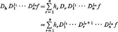
by Theorem 2.2 and the above remarks. It follows that the iterated directional derivative D_h^k f = D_h · · · D_hf exists, with

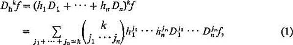
the summation being taken over all n-tuples j₁, . . . , j_n of nonnegative integers whose sum is k. Here the symbol

denotes the “multinomial coefficient” appearing in the general multinomial formula

Actually

see Exercise 7.2.

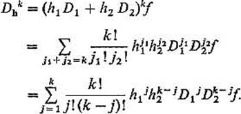
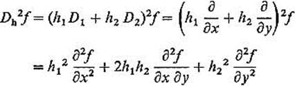
For example, if n = 2 we have ordinary binomial coefficients and (1) gives

For instance, we obtain

and

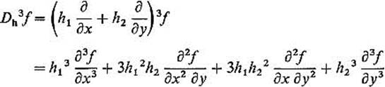
with k = 2 and k = 3, respectively.

These iterated directional derivatives are what we need to state the multidimensional Taylor‘s formula. To see why this should be, consider the 1-dimensional Taylor’s formula in the form

given in Theorem 6.1. Since f^(r)(a)h^r = h^r D₁^r f(a) = (h D₁)^rf(a) = D_hf(a) by Theorem 2.2 with n = 1, so that D_h = hD₁, (2) can be rewritten

where D_h⁰f(a) = f(a). But now (3) is a meaningful equation if f is a real-valued function on ⁿ. If f is of class in a neighborhood of a, then we see from Eq. (1) above that

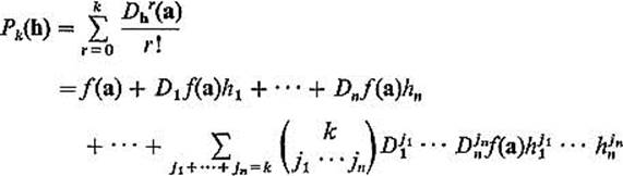
is a polynomial of degree at most k in the components h₁, . . . , h_n of h. Therefore P_k(h) is called the kth degree Taylor polynomial of f at a. The kth degree remainder of f at a is defined by

The notation P_k(h) and R_k(h) is incomplete, since it contains explicit reference to neither the function f nor the point a, but this will cause no confusion in what follows.

Theorem 7.1 (Taylor's Formula) If f is a real-valued function of class ⁺¹ on an open set containing the line segment L from a to a + h, then there exists a point such that

so

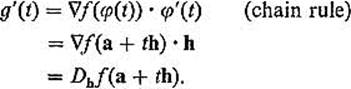
PROOF If φ : is defined by

and g(t) = f(φ(t)) = f(a + th), then g(0) = f(a), g(1) = f(a + h), and Taylor's formula in one variable gives

for some c.(0,1) To complete the proof, it therefore suffices to show that

for r k+1, because then we have

and with (see Fig. 2.38).

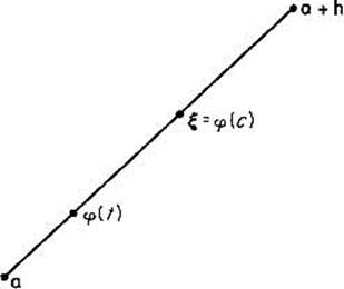
Figure 2.38

Actually, in order to apply the single-variable Taylor's formula, we need to know that g is of class ⁺¹ on [0, 1], but this will follow from (4) because f is of class ⁺¹.

Note first that

Then assume inductively that (4) holds for r k, and let f₁(x) = D_h^rf(x). Then g^(r) = f₁ φ, so

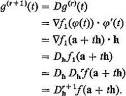
Thus (4) holds by induction for r k + 1 as desired.

If we write x = a + h, then we obtain

where P_k(x − a) is a kth degree polynomial in the components x₁ − a₁, x₂ − a₂, . . . , x_n − a_n of h = x − a, and

for some .

Example 1 Let . Then each , so

Hence the kth degree Taylor polynomial of is

as expected.

Example 2 Suppose we want to expand f(x, y) = xy in powers of x − 1 and y − 1. Of course the result will be

but let us obtain this result by calculating the second degree Taylor polynomial P₂(h) of f(x, y) at a = (1, 1) with h = (h₁, h₂) = (x − 1, y − 1). We will then have f(x, y) = P₂(x − 1, y − 1), since R₃(h) = 0 because all third order partial derivatives of f vanish. Now

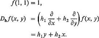
So D_hf(1, 1) = h₁ + h₂ = (x − 1) + (y − 1), and

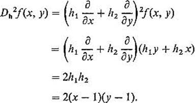
Hence

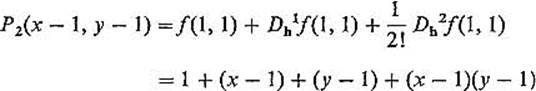
as predicted.

Next we generalize the error estimate of Corollary 6.2.

Corollary 7.2 If f is of class ^{+ 1} in a neighborhood U of a, and R_k(h) is the kth degree remainder of f at a, then

PROOF If h is sufficiently small that the line segment from a to a + h lies in U, then Theorem 7.1 gives

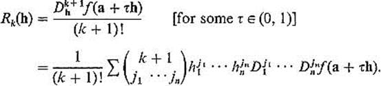
But because f is of class ^{+ 1} It therefore suffices to see that

if j₁ + · · · + j_n = k + 1. But this is so because each , and there is one more factor in the numerator than in the denominator.

Rewriting the conclusion of Corollary 7.2 in terms of the kth degree Taylor polynomial, we have

We shall see that this result characterizes P_k(x − a); that is, P_k(x − a) is the only kth degree polynomial in x₁ − a₁, . . . , x_n − a_n satisfying condition (5).

Lemma 7.3 If Q(x) and Q^*(x) are two kth degree polynomials in x₁, . . . , x_n such that

then Q = Q^*.

PROOF Supposing to the contrary that Q ≠ Q^*, let

where F(x) is the polynomial consisting of all those terms of the lowest degree l which actually appear in Q(x) − Q^*(x), and G(x) consists of all those terms of degree higher than l.

Choose a fixed point b ≠ 0 such that F(b) ≠ 0. Since for t sufficiently small, we have

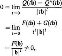
since each term of F is of degree l, while each term of G is of degree > l. This contradiction proves that Q = Q^*.

We can now establish the converse to Corollary 7.2.

Theorem 7.4 If f : is of class ⁺¹ in a neighborhood of a, and Q is a polynomial of degree k such that

then Q is the kth degree Taylor polynomial of f at a.

PROOF Since

by the triangle inequality, (5) and (6) imply that

Since Q and P_k are both kth degree polynomials, Lemma 7.3 gives Q = P_k as desired.

The above theorem can often be used to discover Taylor polynomials of a function when the explicit calculation of its derivatives is inconvenient. In order to verify that a given kth degree polynomial Q is the kth degree Taylor polynomial of the class ⁺¹ function f at a, we need only verify that Q satisfies condition (6).

Example 3 We calculate the third degree Taylor polynomial of e^x sin x by multiplying together those of e^x and sin x. We know that

where lim_x→0 R(x)/x³ = lim_x→0 (x)/x³ = 0. Hence

where

Since it is clear that

it follows from Theorem 7.4 that is the third degree Taylor polynomial of e^x sin x at 0.

Example 4 Recall that

If we substitute t = x and t = y, and multiply the results, we obtain

where

Since it is easily verified that

it follows from Theorem 7.4 that is the second degree Taylor polynomial of e^x+y at (0, 0).

We shall next give a first application of Taylor polynomials to multivariable maximum-minimum problems. Given a critical point a for f : , we would like to have a criterion for determining whether f has a local maximum or a local minimum, or neither, at a. If f is of class in a neighborhood of a, we can write its second degree Taylor expansion in the form

where

and

If not all of the second partial derivatives of f vanish at a, then q(h) is a (non-trivial) homogeneous second degree polynomial in h₁, . . . , h_n of the form

and is called the quadratic form of f at the critical point a. Note that

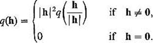
Since h/h is a point of the unit sphere Sⁿ⁻¹ in ⁿ, it follows that the quadratic form q is completely determined by its values on Sⁿ⁻¹. As in the 2-dimensional case of Section 4, a quadratic form is called positive-definite(respectively negative-definite) if and only if it is positive (respectively negative) at every point of Sⁿ⁻¹ (and hence everywhere except 0), and is called nondefinite if it assumes both positive and negative values on Sⁿ⁻¹ (and hence in every neighborhood of 0).

For example, x² + y² is positive-definite and −x² − y² is negative-definite, while x² − y² and xy are nondefinite. Note that y², regarded as a quadratic form in x and y whose coefficients of both x² and xy are zero, is neither positive-definite nor negative-definite nor nondefinite (it is not negative anywhere, but is zero on the x-axis).

In the case n = 1, when f is a function of a single variable with critical point a, the quadratic form of f at a is simply

Note that q is positive-definite if f′(a) > 0, and is negative-definite if f′(a) < 0 (the nondefinite case cannot occur if n = 1). Therefore the “second derivative test” for a single-variable function states that f has a local minimum at a if its quadratic form q(h) at a is positive-definite, and a local maximum at a if q(h) is negative-definite. If f′(a) = 0, then q(h) = 0 is neither positive-definite nor negative-definite (nor nondefinite), and we cannot determine (without considering higher derivatives) the character of the critical point a. The following theorem is the multivariable generalization of the “second derivative test.”

Theorem 7.5 Let f be of class in a neighborhood of the critical point a. Then f has

(a)a local minimum at a if its quadratic form q(h) is positive-definite,

(b)a local maximum at a if q(h) is negative-definite,

(c)neither if q(h) is nondefinite.

PROOF Since f(a + h) − f(a) = q(h) + R₂(h), it suffices for (a) to find a Δ > 0 such that

Note that

Since is a closed and bounded set, q(h/h) attains a minimum value m, and m > 0 because q is positive-definite. Then

But lim_h→0 R₂(h)/h² = 0, so there exists Δ > 0 such that

Then

as desired.

The proof for case (b) is similar.

If q(h) is nondefinite, choose two fixed points h₁ and h₂ in ⁿ such that q(h₁) > 0 and q(h₂) < 0. Then

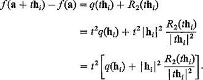
Since lim_t→0 R₂(th_i)/th_i² = 0, it follows that, for t sufficiently small, f(a + th_i) − f(a) is positive if i = 1, and negative if i = 2. Hence f has neither a local minimum nor a local maximum at a.

For example, suppose that a is a critical point of f(x, y). Then f has a local minimum at a if q(x, y) = x² + y², a local maximum at a if q(x, y) = −x² − y², and neither if q(x, y) = x² − y². If q(x, y) = y² or q(x, y) = 0, then see Theorem 7.5 does not apply. In the cases where the theorem does apply, it says simply that the character of f at a is the same as that of q at 0 (Fig. 2.39).

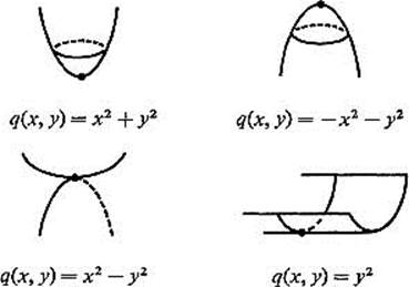
Figure 2.39

Example 5 Let f(x, y) = x² + y² + cos x. Then (0, 0) is a critical point of f. Since

Theorem 7.4 implies that the second degree Taylor polynomial of f at (0, 0) is

so the quadratic form of f at (0, 0) is

Since q(x, y) is obviously positive-definite, it follows from Theorem 7.5 that f has a local minimum at (0, 0).

Example 6 The point a = (2, π/2) is a critical point for the function f(x, y) = x² sin y − 4x. Since

the second degree Taylor expansion of f at (2, π/2) is

Consequently the quadratic form of f at (2, π/2) is defined by

(writing q in terms of x and y through habit). Since q is clearly nondefinite, it follows from Theorem 7.5 that f has neither a local maximum nor a local minimum at (2, π/2).

Consequently, in order to determine the character of the critical point a of f, we need to maximize and minimize its quadratic form on the unit sphere Sⁿ⁻¹. This is a Lagrange multiplier problem with which we shall deal in the next section.

Exercises

7.1If f is a function of class , and i₁′, . . . , i_q′ is a permutation of i₁, . . . , i_q, prove by induction on q that

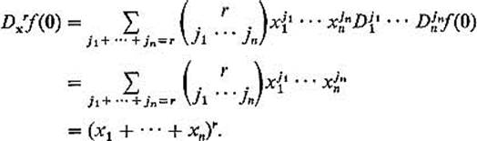
7.2Let f(x) = (x₁ + · · · + x_n)^k.

(a)Show that .

(b)Show that

(c)Conclude that

7.3Find the third degree Taylor polynomial of f(x, y) = (x + y)³ at (0, 0) and (1, 1).

7.4Find the third degree Taylor polynomial of f(x, y, z) = xy²z³ at (1, 0, −1).

7.5Assuming the facts that the sixth degree Taylor polynomials of tan⁻¹ x and sin² x are

respectively, use Theorem 7.4 to show that the sixth degree Taylor polynomial of

at 0 is . Why does it now follow from Theorem 6.3 that f has a local minimum at 0?

7.6Let f(x, y) = e^xy sin(x + y). Multiply the Taylor expansions

and

together, and apply Theorem 7.4 to show that

is the third degree Taylor polynomial of f at 0. Conclude that

7.7Apply Theorem 7.4 to prove that the Taylor polynomial of degree 4n + 1 for f(x) = sin(x²) at 0 is

Hint: sin x = P_2n+1(x) + R_2n+1(x), where

Hence lim_x→0 R_2n+1(x²)/x⁴ⁿ⁺¹ = 0.

7.8Apply Theorem 7.4 to show that the sixth degree Taylor polynomial of f(x) = sin² x at 0 is .

7.9Apply Theorem 7.4 to prove that the kth degree Taylor polynomial of f(x)g(x) can be obtained by multiplying together those of f(x) and g(x), and then deleting from the product all terms of degree greater than k.

7.10Find and classify the critical points of .

7.11Classify the critical point (−1, π/2, 0) of f(x, y, z) = x sin z − z sin y.

7.12Use the Taylor expansions given in Exercises 7.5 and 7.6 to classify the critical point (0, 0, 0) of the function f(x, y, z) = x² + y² + e^xy − y tan⁻¹ x + sin² z.