Advanced Calculus of Several Variables (1973)
Part II. Multivariable Differential Calculus
Chapter 8. THE CLASSIFICATION OF CRITICAL POINTS
Let f be a real-valued function of class ![]() on an open set
on an open set ![]() , and let
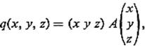
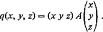
, and let ![]() be a critical point of f. In order to apply Theorem 7.5 to determine the nature of the critical point a, we need to decide the character of the quadratic form
be a critical point of f. In order to apply Theorem 7.5 to determine the nature of the critical point a, we need to decide the character of the quadratic form ![]() defined by
defined by
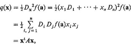
where the n × n matrix A = (aij) is defined by ![]() , and
, and
Note that the matrix A is symmetric, that is aij = aji, since Di Dj = Dj Di.
We have seen that, in order to determine whether q is positive-definite, negative-definite, or nondefinite, it suffices to determine the maximum and minimum values of q on the unit sphere Sn−1. The following result rephrases this problem in terms of the linear mapping ![]() defined by
defined by
![]()
We shall refer to the quadratic form q, the symmetric matrix A, and the linear mapping L as being “associated” with one another.
Theorem 8.1 If the quadratic form q attains its maximum or minimum value on Sn−1 at the point ![]() , then there exists a real number λ such that
, then there exists a real number λ such that
![]()
where L is the linear mapping associated with q.
Such a nonzero vector v, which upon application of the linear mapping ![]() is simply multiplied by some real number λ, L(v) = λv, is called an eigenvector of L, with associated eigenvalue λ.
is simply multiplied by some real number λ, L(v) = λv, is called an eigenvector of L, with associated eigenvalue λ.
PROOF We apply the Lagrange multiplier method. According to Theorem 5.5, there exists a number ![]() such that
such that
![]()
where ![]() defines the sphere Sn−1.
defines the sphere Sn−1.
But Dk g(x) = 2xk, and
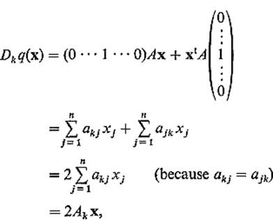
where the row vector Ak is the kth row of A, that is, Ak = (ak1 · · · akn). Consequently Eq. (1) implies that
![]()
for each i = 1, . . . , n. But Ak v is the ith row of Av, while λvk is the kth element of the column vector λv, so we have
![]()
as desired.
![]()
Thus the problem of maximizing and minimizing q on Sn−1 involves the eigenvectors and eigenvalues of the associated linear mapping. Actually, it will turn out that if we can determine the eigenvalues without locating the eigenvectors first, then we need not be concerned with the latter.
Lemma 8.2 If ![]() is an eigenvector of the linear mapping
is an eigenvector of the linear mapping ![]() associated with the quadratic form q, then
associated with the quadratic form q, then
![]()
where λ is the eigenvalue associated with v.
PROOF
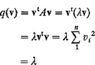
since ![]() .
.
![]()
The fact that we need only determine the eigenvalues of L (and not the eigenvectors) is a significant advantage, because the following theorem asserts that we therefore need only solve the so-called characteristic equation
![]()
Here ![]() A − λI
A − λI![]() denotes the determinant of the matrix A − λI (where I is the n × n identity matrix).
denotes the determinant of the matrix A − λI (where I is the n × n identity matrix).
Theorem 8.3 The real number λ is an eigenvalue of the linear mapping ![]() , defined by L(x) = Ax, if and only if λ satisfies the equation
, defined by L(x) = Ax, if and only if λ satisfies the equation
![]()
PROOF Suppose first that λ is an eigenvalue of L, that is,
![]()
for some v ≠ 0. Then (A − λI)v = 0.
Enumerating the rows of the matrix A − λI, we obtain
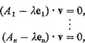
where e1, . . . , en are the standard unit vectors in ![]() n. Hence the n vectors A1 − λe1, . . . , An − λen all lie in the (n − 1)-dimensional hyperplane through 0 perpendicular to v, and are therefore linearly dependent, so it follows from Theorem I.6.1 that
n. Hence the n vectors A1 − λe1, . . . , An − λen all lie in the (n − 1)-dimensional hyperplane through 0 perpendicular to v, and are therefore linearly dependent, so it follows from Theorem I.6.1 that
![]()
as desired.
Conversely, if λ is a solution of ![]() A − λI
A − λI![]() = 0, then the row vectors A1 − λe1, . . . , An − λen of A − λI are linearly dependent, and therefore all lie in some (n − 1)-dimensional hyperplane through the origin. If v is a unit vector perpendicular to this hyperplane, then
= 0, then the row vectors A1 − λe1, . . . , An − λen of A − λI are linearly dependent, and therefore all lie in some (n − 1)-dimensional hyperplane through the origin. If v is a unit vector perpendicular to this hyperplane, then
![]()
Hence (A − λI)v = 0, so
![]()
as desired.
![]()
Corollary 8.4 The maximum (minimum) value attained by the quadratic form q(x) = xtAx on Sn−1 is the largest (smallest) real root of the equation
![]()
PROOF If q(v) is the maximum (minimum) value of q on Sn−1, then v is an eigenvector of L(x) = Ax by Theorem 8.1, and q(v) = λ, the associated eigenvalue, by Lemma 8.2. Theorem 8.3 therefore implies that q(v) is a root of ![]() A − λI
A − λI![]() = 0. On the other hand, it follows from 8.2 and 8.3 that every root of
= 0. On the other hand, it follows from 8.2 and 8.3 that every root of ![]() A − λI
A − λI![]() = 0 is a value of q on Sn−1. Consequently q(v) must be the largest (smallest) root of
= 0 is a value of q on Sn−1. Consequently q(v) must be the largest (smallest) root of ![]() A − λI
A − λI![]() = 0.
= 0.
![]()
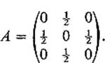
Example 1 Suppose a is a critical point of the function f: ![]() and that the quadratic form of f at a is
and that the quadratic form of f at a is
![]()
so the matrix of q is
![]()
The characteristic equation of A is then
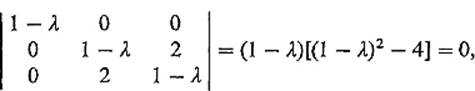
with roots λ = −1, 1, 3. It follows from Corollary 8.4 that the maximum and minimum values of q in S2 are + 3 and − 1 respectively. Since q attains both positive and negative values, it is nondefinite. Hence Theorem 7.5 implies that f has neither a maximum nor a minimum at a.
The above example indicates how Corollary 8.4 reduces the study of the quadratic form q(x) = xtAx to the problem of finding the largest and smallest real roots of the characteristic equation ![]() A − λI
A − λI![]() = 0. However this problem itself can be difficult. It is therefore desirable to carry our analysis of quadratic forms somewhat further.
= 0. However this problem itself can be difficult. It is therefore desirable to carry our analysis of quadratic forms somewhat further.
Recall that the matrix A of a quadratic form is symmetric, that is, aij = aji. We say that the linear mapping ![]() is symmetric if and only if L(x) · y = x · L(y) for all x and y in
is symmetric if and only if L(x) · y = x · L(y) for all x and y in ![]() n. The motivation for this terminology is the following result.
n. The motivation for this terminology is the following result.
Lemma 8.5 If A is the matrix of the linear mapping ![]() , then L is symmetric if and only if A is symmetric.
, then L is symmetric if and only if A is symmetric.
PROOF If ![]() , then
, then
![]()
Hence L is symmetric if and only if
![]()
for all i, j = 1, . . . , n. But
![]()
and![]()
The following theorem gives the precise character of a quadratic form q in terms of the eigenvectors and eigenvalues of its associated linear mapping L.
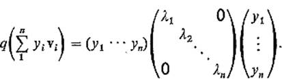
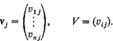
Theorem 8.6 If q is a quadratic form on ![]() n, then there exists an orthogonal set of unit eigenvectors v1, . . . , vn of the associated linear mapping L. If y1, . . . , yn are the coordinates of
n, then there exists an orthogonal set of unit eigenvectors v1, . . . , vn of the associated linear mapping L. If y1, . . . , yn are the coordinates of ![]() with respect to the basis v1, . . . , vn, that is,
with respect to the basis v1, . . . , vn, that is,
![]()
then
![]()
where λ1, . . . , λn are the eigenvalues of v1, . . . , vn.
PROOF This is trivially true if n = 1, for then q is of the form q(x) = λx2, with L(x) = λx. We therefore assume by induction that it is true in dimension n − 1.
If q attains its maximum value on the unit sphere Sn−1 at ![]() , then see Theorem 8.1 says that vn is an eigenvector of L. Fig. 2.40.
, then see Theorem 8.1 says that vn is an eigenvector of L. Fig. 2.40.
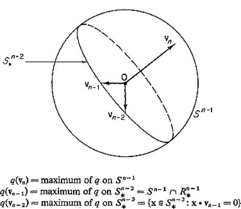
Figure 2.40
Let ![]() be the subspace of
be the subspace of ![]() n perpendicular to vn. Then L maps
n perpendicular to vn. Then L maps ![]() into itself, because, given
into itself, because, given ![]() , we have
, we have
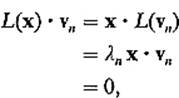
using the symmetry of L (Lemma 8.5).
Let ![]() and
and ![]() be the “restrictions” of L and q to
be the “restrictions” of L and q to ![]() , that is,
, that is,
![]()
If (u1, . . . , un−1) are the coordinates of x with respect to an orthonormal basis for ![]() n−1, then by Lemma 8.5,
n−1, then by Lemma 8.5,
![]()
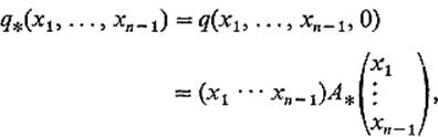
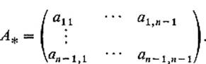
where B is a symmetric (n − 1) × (n − 1) matrix. Then
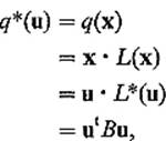
so q* is a quadratic form in u1, . . . , un−1.
The inductive hypothesis therefore gives an orthogonal set of unit eigenvectors v1, . . . , vn−1 for L*. Then v1, . . . , vn is the desired orthogonal set of unit eigenvectors for L.
To prove the last statement of the theorem, let ![]() . Then
. Then
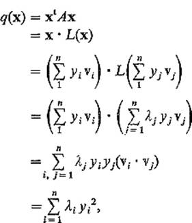
since vi · vj = 0 unless i = j, and vi · vi = 1.
![]()
Equation (2) may be written in the form
The process of finding an orthogonal set of unit eigenvectors, with respect to which the matrix of q is diagonal, is sometimes called diagonalization of the quadratic form q.
Note that, independently of Corollary 8.4, it follows immediately from Eq. (2) that
(a)q is positive-definite if all the eigenvalues are positive,
(b)q is negative-definite if all the eigenvalues are negative, and
(c)q is nondefinite if some are positive and some are negative.
If one or more eigenvalues are zero, while the others are either all positive or all negative, then q is neither positive-definite nor negative-definite nor nondefinite. According to Lemma 8.7 below, this can occur only if the determinant of the matrix of q vanishes.
Example 2 If q(x, y, z) = xy + yz, the matrix of q is
The characteristic equation is then
![]()
with solutions ![]() . By substituting each of these eigenvalues in turn into the matrix equation
. By substituting each of these eigenvalues in turn into the matrix equation
![]()
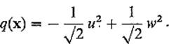
(from the proof of Theorem 8.3), and solving for a unit vector v, we obtain the eigenvectors
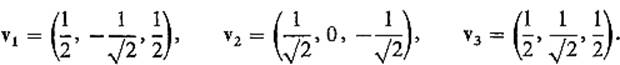
If u, v, w are coordinates with respect to coordinate axes determined by v1, v2, v3, that is, x = uv1 + vv2 + wv3, then Eq. (2) gives
Lemma 8.7 If λ1, . . . , λn are eigenvalues of the symmetric n × n matrix A, corresponding to orthogonal unit eigenvectors v1, . . . , vn, then
![]()
PROOF Let
Then, since Avj = λivj, we have
![]()
It follows that
![]()
Since ![]() V
V![]() ≠ 0 because the vectors v1, . . . , vn are orthogonal and therefore linearly independent, this gives Eq. (3).
≠ 0 because the vectors v1, . . . , vn are orthogonal and therefore linearly independent, this gives Eq. (3).
![]()
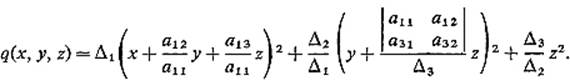
We are finally ready to give a complete analysis of a quadratic form q(x) = xt Ax on ![]() n for which
n for which ![]() A
A![]() ≠ 0. Writing A = (aij) as usual, we denote by Δk the determinant of the upper left-hand k × k submatrix of A, that is,
≠ 0. Writing A = (aij) as usual, we denote by Δk the determinant of the upper left-hand k × k submatrix of A, that is,
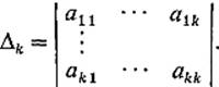
Thus
![]()
Theorem 8.8 Let q(x) = xt Ax be a quadratic form on ![]() n with
n with ![]() A
A![]() ≠ 0. Then q is
≠ 0. Then q is
(a)positive-definite if and only if Δk >0 for each k = 1, . . . , n,
(b)negative-definite if and only if (−1)k Δk >0 for each k = 1, . . . , n,
(c)nondefinite if neither of the previous two conditions is satisfied.
PROOF OF (a) This is obvious if n = 1; assume by induction its truth in dimension n − 1.
Since 0 < Δn = ![]() A
A![]() = λ1λ2 · · · λn by Lemma 8.7, all the eigenvalues λ1, . . . , λn of A are nonzero. Either they are all positive, in which case we are finished, or an even number of them are negative. In the latter case, let λi and λj be two negative eigenvalues, corresponding to eigenvectors vi and vj.
= λ1λ2 · · · λn by Lemma 8.7, all the eigenvalues λ1, . . . , λn of A are nonzero. Either they are all positive, in which case we are finished, or an even number of them are negative. In the latter case, let λi and λj be two negative eigenvalues, corresponding to eigenvectors vi and vj.
Let ![]() be the 2-plane in
be the 2-plane in ![]() n spanned by vi and vj. Then, given
n spanned by vi and vj. Then, given ![]() , we have
, we have

so q is negative on ![]() minus the origin.
minus the origin.
Now let q* : ![]() n − 1
n − 1 ![]() be the restriction of q to
be the restriction of q to ![]() n−1, defined by
n−1, defined by
where
Since Δ1 >0, . . . , Δn − 1 >0, the inductive assumption implies that q* is positive-definite on ![]() n−1. But this is a contradiction, since the (n − 1)-plane
n−1. But this is a contradiction, since the (n − 1)-plane ![]() n−1 and the 2-plane
n−1 and the 2-plane ![]() , on which q is negative, must have at least a line in common. We therefore conclude that q has no negative eigenvalues, and hence is positive-definite.
, on which q is negative, must have at least a line in common. We therefore conclude that q has no negative eigenvalues, and hence is positive-definite.
Conversely, if q is positive-definite, we want to prove that each Δk is positive. If m is the minimum value of q on Sn−1, then m >0.
Let qk : ![]() k
k ![]() be the restriction of q to
be the restriction of q to ![]() k, that is,
k, that is,
where Ak is the upper left-hand k × k submatrix of A, so Δk = ![]() Ak
Ak![]() , and define Lk :
, and define Lk : ![]() k
k ![]() k by Lk(x) = Ak x. Then Lk is symmetric by Lemma 8.5.
k by Lk(x) = Ak x. Then Lk is symmetric by Lemma 8.5.
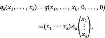
Let ¼1, . . . , ¼k be the eigenvalues of Lk given by Theorem 8.6. Since by Lemma 8.2 each ¼i is the value of qk at some point of Sk−1, the unit sphere in ![]() k, and qk(x) = q(x, 0), it follows that each
k, and qk(x) = q(x, 0), it follows that each ![]() . Finally Lemma 8.7implies that
. Finally Lemma 8.7implies that
![]()
PROOF OF (b) Define the quadratic form q* : ![]() n
n ![]() by q*(x) = −q(x). Then clearly q is negative-definite if and only if q* is positive-definite. By part (a), q* is positive-definite if and only if each Δk* is positive, where Δk* =
by q*(x) = −q(x). Then clearly q is negative-definite if and only if q* is positive-definite. By part (a), q* is positive-definite if and only if each Δk* is positive, where Δk* = ![]() −Ak
−Ak![]() , Ak being the upper left-hand k × k submatrix of A. But, since each of the k rows of − Ak is −1 times the corresponding row of Ak, it follows that
, Ak being the upper left-hand k × k submatrix of A. But, since each of the k rows of − Ak is −1 times the corresponding row of Ak, it follows that
![]()
PROOF OF (c) Since Δn = λ1 λ2 · · · λn ≠ 0, all of the eigenvalues λ1, . . . , λn are nonzero. If all of them were positive, then part (a) would imply that Δk >0 for all k, while if all of them were negative, then part (b) would imply that (−1)k Δk >0 for all k. Since neither is the case, we conclude that q has both positive eigenvalues and negative eigenvalues, and is therefore nondefinite.
![]()
Recalling that, if a is a critical point of the class ![]() function f :
function f : ![]() , the quadratic form of f at a is
, the quadratic form of f at a is ![]() , Theorems 7.5 and 8.8 enable us to determine the behavior of f in a neighborhood of a,provided that the determinant
, Theorems 7.5 and 8.8 enable us to determine the behavior of f in a neighborhood of a,provided that the determinant
![]()
often called the Hessian determinant of f at a, is nonzero. But if ![]() Di Djf(a)
Di Djf(a)![]() = 0, then these theorems do not apply, and ad hoc methods must be applied.
= 0, then these theorems do not apply, and ad hoc methods must be applied.
Note that the classical second derivative test for a function of two variables (Theorem 4.4) is an immediate corollary to Theorems 7.5 and 8.8.
It will clarify the picture at this point to generalize the discussion at the end of Section 6. Suppose for the sake of simplicity that the origin is a critical point of the class ![]() function f:
function f: ![]() , and that f(0) = 0. Then
, and that f(0) = 0. Then
![]()
with
![]()
Let v1, . . . , vn be an orthogonal set of unit eigenvectors (provided by Theorem 8.6), with associated eigenvalues λ1, . . . , λn. Assume that ![]() Di Djf(0)
Di Djf(0)![]() ≠ 0, so Lemma 8.7 implies that each λi is nonzero. Let λ1, . . . , λk be the positive eigenvalues, and λk+1, . . . , λn the negative ones (writing k = 0 if all the eigenvalues are negative). Since
≠ 0, so Lemma 8.7 implies that each λi is nonzero. Let λ1, . . . , λk be the positive eigenvalues, and λk+1, . . . , λn the negative ones (writing k = 0 if all the eigenvalues are negative). Since
![]()
if x = y1v1 + · · · + yn vn, it is clear that q has a minimum at 0 if k = n and a maximum if k = 0.
If ![]() , so that q has both positive and negative eigenvalues, denote by
, so that q has both positive and negative eigenvalues, denote by ![]() the subspace of
the subspace of ![]() spanned by v1, . . . , vk, and by
spanned by v1, . . . , vk, and by ![]() the subspace of
the subspace of ![]() n spanned by vk+1, . . . , vn. Then the graph of z = q(x) in
n spanned by vk+1, . . . , vn. Then the graph of z = q(x) in ![]() and
and ![]() looks like Fig. 2.41; q has a minimum on
looks like Fig. 2.41; q has a minimum on ![]() and a maximum on
and a maximum on ![]() .
.
Given ![]() < mini
< mini ![]() λi
λi![]() , choose δ >0 such that
, choose δ >0 such that
![]()
or
![]()
since ![]() . This inequality and Eq. (4) yield
. This inequality and Eq. (4) yield
![]()
Using (5), we obtain
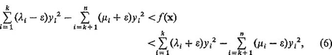
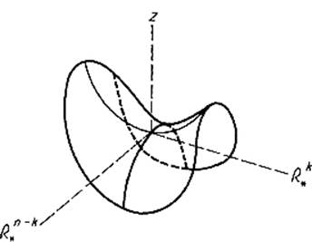
Figure 2.41
where ¼i = −λi >0, i = k + 1, . . . , n. Since λi − ![]() >0 and ¼i −
>0 and ¼i − ![]() >0 because
>0 because ![]() < min
< min ![]() λi
λi![]() , inequalities (6) show that, for
, inequalities (6) show that, for ![]() x
x![]() < δ, the graph of z = f(x) lies between two very close quadratic surfaces (hyperboloids) of the same type as z = q(x). In particular, if
< δ, the graph of z = f(x) lies between two very close quadratic surfaces (hyperboloids) of the same type as z = q(x). In particular, if ![]() , then f has a local minimum on the subspace
, then f has a local minimum on the subspace ![]() and a local maximum on the subspace
and a local maximum on the subspace  . This makes it clear that the origin is a “saddle point” for f if q has both positive and negative eigenvalues. Thus the general case is just like the 2-dimensional case except that, when there is a saddle point, the subspace on which the critical point is a maximum point may have any dimension from 1 to n − 1.
It should be emphasized that, if the Hessian determinant ![]() DiDjf(a)
DiDjf(a)![]() is zero, then the above results yield no information about the critical point a. This will be the situation if the quadratic form q of f at a is either positive-semidefinite but not positive-definite, or negative-semidefinite but not negative-definite. The quadratic form q is called positive-semidefinite if
is zero, then the above results yield no information about the critical point a. This will be the situation if the quadratic form q of f at a is either positive-semidefinite but not positive-definite, or negative-semidefinite but not negative-definite. The quadratic form q is called positive-semidefinite if ![]() for all x, and negative-semidefinite if
for all x, and negative-semidefinite if ![]() for all x. Notice that the terminology “q is nondefinite,” which we have been using, actually means that q is neither positive-semidefinite nor negative-semidefinite (so we might more descriptively have said “ nonsemidefinite”).
for all x. Notice that the terminology “q is nondefinite,” which we have been using, actually means that q is neither positive-semidefinite nor negative-semidefinite (so we might more descriptively have said “ nonsemidefinite”).
Example 3 Let f(x, y) = x2 − 2xy + y2 + x4 + y4, and g(x, y) = x2 − 2xy + y2 − x4 − y4. Then the quadratic form for both at the critical point (0, 0) is
![]()
which is positive-semidefinite but not positive-definite. Since
![]()
f has a relative minimum at (0, 0). However, since
![]()
it is clear that g has a saddle point at (0, 0).
Thus, if the Hessian determinant vanishes, then anything can happen.
We conclude this section with discussion of a “second derivative test” for constrained (Lagrange multiplier) maximum–minimum problems. We first recall the setting for the general Lagrange multiplier problem: We have a differentiable function f: ![]() and a continuously differentiable mapping G :
and a continuously differentiable mapping G : ![]() m (m < n), and denote by M the set of all those points
m (m < n), and denote by M the set of all those points ![]() at which the gradient vectors ∇G1(x), . . . , ∇Gm(x), of the component functions of G, are linearly independent. By Theorem 5.7, M is an (n − m)-dimensional manifold in
at which the gradient vectors ∇G1(x), . . . , ∇Gm(x), of the component functions of G, are linearly independent. By Theorem 5.7, M is an (n − m)-dimensional manifold in ![]() n, and by Theorem 5.6 has an (n − m)-dimensional tangent space Tx at each point
n, and by Theorem 5.6 has an (n − m)-dimensional tangent space Tx at each point ![]() . Recall that, by definition, Tx is the subspace of
. Recall that, by definition, Tx is the subspace of ![]() n consisting of all velocity vectors (at x) to differentiable curves on M which pass through x. This notation will be maintained throughout the present discussion.
n consisting of all velocity vectors (at x) to differentiable curves on M which pass through x. This notation will be maintained throughout the present discussion.
We are interested in locating and classifying those points of M at which the function f attains its local maxima and minima on M. According to see Theorem 5.1, in order for f to have a local maximum or minimum on M at ![]() , it is necessary that a be a critical point for f on M in the following sense. The point
, it is necessary that a be a critical point for f on M in the following sense. The point ![]() is called a critical point for f on M if and only if the gradient vector ∇f(a) is orthogonal to the tangent space Ta of M at a. Since the linearly independent gradient vectors ∇G1(a), . . . , ∇Gm(a) generate the orthogonal complement to Ta (Fig. 2.42), it follows as in Theorem 5.8 that there exist unique numbers λ1, . . . , λm such that
is called a critical point for f on M if and only if the gradient vector ∇f(a) is orthogonal to the tangent space Ta of M at a. Since the linearly independent gradient vectors ∇G1(a), . . . , ∇Gm(a) generate the orthogonal complement to Ta (Fig. 2.42), it follows as in Theorem 5.8 that there exist unique numbers λ1, . . . , λm such that
![]()
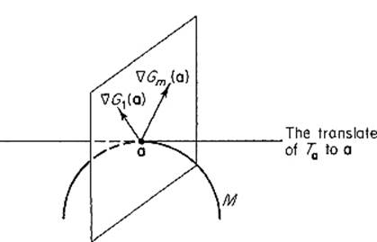
Figure 2.42
We will obtain sufficient conditions for f to have a local extremum at a by considering the auxiliary function H : ![]() for f at a defined by
for f at a defined by
![]()
Notice that (7) simply asserts that ∇H(a) = 0, so a is an (ordinary) critical point for H. We are, in particular, interested in the quadratic form
![]()
of H at a.
Theorem 8.9 Let a be a critical point for f on M, and denote by q : ![]() the quadratic form at a of the auxiliary function
the quadratic form at a of the auxiliary function ![]() , as above. If f and G are both of class
, as above. If f and G are both of class ![]() in a neighborhood of a, then f has
in a neighborhood of a, then f has
(a)a local minimum on M at a if q is positive-definite on the tangent space Ta to M at a,
(b)a local maximum on M at a if q is negative-definite on Ta,
(c)neither if q is nondefinite on Ta.
The statement, that “q is positive-definite on Ta,” naturally means that q(h) >0 for all nonzero vectors ![]() ; similarly for the other two cases.
; similarly for the other two cases.
PROOF The proof of each part of this theorem is an extension of the proof of the corresponding part of Theorem 7.5. We give the details only for part (a).
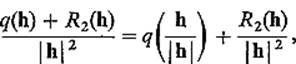
We start with the Taylor expansion
![]()
for the auxiliary function H. Since ![]() , it clearly suffices to find a δ >0 such that
, it clearly suffices to find a δ >0 such that
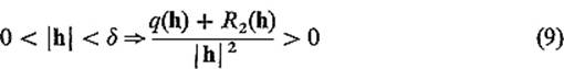
if![]()
Let m be the minimum value attained by q on the unit sphere ![]() in the tangent plane Ta. Then m >0 because q is positive-definite on Ta. Noting that
in the tangent plane Ta. Then m >0 because q is positive-definite on Ta. Noting that
we choose δ >0 so small that
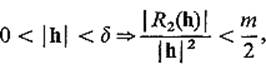
and also so small that 0 < ![]() h
h![]() < δ and
< δ and ![]() together imply that h/
together imply that h/![]() h
h![]() is sufficiently near to S* that
is sufficiently near to S* that
![]()
Then (9) follows as desired. The latter condition on δ can be satisfied because S* is (by definition) the set of all tangent vectors at a to unit-speed curves on M which pass through a. Therefore, if ![]() and h is sufficiently small, it follows that h/
and h is sufficiently small, it follows that h/![]() h
h![]() is close to a vector in S*.
is close to a vector in S*.
![]()
The following two examples provide illustrative applications of Theorem 8.9.
Example 4 In Example 4 of Section 5 we wanted to find the box with volume 1000 having least total surface area, and this involved minimizing the function
![]()
on the 2-manifold ![]() defined by the constraint equation
defined by the constraint equation
![]()
We found the single critical point a = (10, 10, 10) for f on M, with ![]() . The auxiliary function is then defined by
. The auxiliary function is then defined by
![]()
We find by routine computation that the matrix of second partial derivatives of h at a is
so the quadratic form of h at a is
![]()
It is clear that q is nondefinite on ![]() 3. However it is the behavior of q on the tangent plane Ta that interests us.
3. However it is the behavior of q on the tangent plane Ta that interests us.
Since the gradient vector ∇g(a) = (100, 100, 100) is orthogonal to M at a = (10, 10, 10), the tangent plane Ta is generated by the vectors
![]()
Given ![]() , we may therefore write
, we may therefore write
![]()
and then find by substitution into (10) that
![]()
Since the quadratic form s2 + st + t2 is positive-definite (by the ac − b2 test), it follows that q is positive-definite on Ta. Therefore Theorem 8.9 assures us that f does indeed have a local minimum on M at the critical point a = (10, 10, 10).
Example 5 In Example 9 of Section 5 we sought the minimum distance between the circle x2 + y2 = 1 and the straight line x + y = 4. This involved minimizing the function
![]()
on the 2-manifold ![]() defined by the constraint equations
defined by the constraint equations
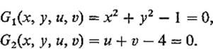
We found the geometrically obvious critical points (see Fig. 2.43), ![]() with
with ![]() It is obvious that f has a minimum at a, and neither a maximum nor a minimum at b, but we want to verify this using Theorem 8.9.
It is obvious that f has a minimum at a, and neither a maximum nor a minimum at b, but we want to verify this using Theorem 8.9.
The auxiliary function H is defined by
![]()
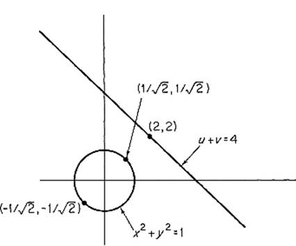
Figure 2.43
By routine computation, we find that the matrix of second partial derivatives of H is
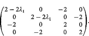
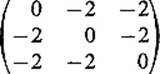
Substituting ![]() , we find that the quadratic form of H at the critical point
, we find that the quadratic form of H at the critical point ![]() is
is
![]()
Computing the subdeterminants Δ1, Δ2, Δ3, Δ4 of Theorem 8.8, we find that all are positive, so this quadratic form q is positive-definite on ![]() 4, and hence on the tangent plane Ta (this could also be verified by the method of the previous example). Hence Theorem 8.9 implies that f does indeed attain a local minimum at a.
4, and hence on the tangent plane Ta (this could also be verified by the method of the previous example). Hence Theorem 8.9 implies that f does indeed attain a local minimum at a.
Substituting ![]() , we find that the quadratic form of H at the other critical point
, we find that the quadratic form of H at the other critical point ![]() is
is
![]()
Now the vectors v1 = (1, −1, 0, 0) and v2 = (0, 0, 1, −1) obviously lie in the tangent plane Tb. Since
![]()
we see that q is nondefinite on Tb, so Theorem 8.9 implies that f does not have a local extremum at b.
Exercises
8.1This exercise gives an alternative proof of Theorem 8.8 in the 3-dimensional case. If
where A = (aij) is a symmetric 3 × 3 matrix with Δ1 ≠ 0, Δ2 ≠ 0, show that
Conclude that q is positive-definite if Δ1, Δ2, Δ3 are all positive, while q is negative-definite if Δ1 < 0, Δ2 >0, Δ3 < 0.
8.2Show that q(x, y, z) = 2x2 + 5y2 + 2z2 + 2xz is positive-definite by
(a)applying the previous exercise,
(b)solving the characteristic equation.
8.3Use the method of Example 2 to diagonalize the quadratic form of Exercise 8.2, and find its eigenvectors. Then sketch the graph of the equation 2x2 + 5y2 + 2z2 + 2xz = 1.
8.4This problem deals with the function ![]() defined by
defined by
![]()
Note that 0 = (0, 0, 0) is a critical point of f.
(a)Show that q(x, y, z) = 2x2 +5y2 + 2z2 + 2xz is the quadratic form of f at 0 by substituting the expansion ![]() , collecting all second degree terms, and verifying the appropriate condition on the remainder
, collecting all second degree terms, and verifying the appropriate condition on the remainder ![]() (x, y, z). State the uniqueness theorem which you apply.
(x, y, z). State the uniqueness theorem which you apply.
(b)Write down the symmetric 3 × 3 matrix A such that
By calculating determinants of appropriate submatrices of A, determine the behavior of f at 0.
(c)Find the eigenvalues λ1, λ2, λ3 of q. Let v1, v2, v3 be the eigenvectors corresponding to λ1, λ2, λ3 (do not solve for them). Express q in the uvw-coordinate system determined by v1, v2, v3. That is, write q(uv1 + uv2 + wv3) in terms of u, v, w. Then give a geometric description (or sketch) of the surface
![]()
8.5Suppose you want to design an ice-cube tray of minimal cost, which will make one dozen ice “cubes” (not necessarily actually cubes) from 12 in.3 of water. Assume that the tray is divided into 12 square compartments in a 2 × 6 pattern as shown in Fig. 2.44, and that
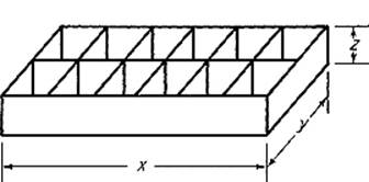
Figure 2.44
the material used costs 1 cent per square inch. Use the Lagrange multiplier method to minimize the cost function f(x, y, z) = xy + 3xz + 7yz subject to the constraints x = 3y and xyz = 12. Apply Theorem 8.9 to verify that you do have a local minimum.
8.6Apply Theorem 8.8 to show that the quadratic form
![]() is nondefinite. Solve the characteristic equation for its eigenvalues, and then find an ortho-normal set of eigenvectors.
is nondefinite. Solve the characteristic equation for its eigenvalues, and then find an ortho-normal set of eigenvectors.
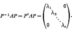
8.7Let f(x) = xt Ax be a quadratic form on ![]() n (with A symmetric), and let v1, . . . , vn be the orthonormal eigenvectors given by Theorem 8.6. If P = (v1, . . . , vn) is the n × n matrix having these eigenvectors as its column vectors, show that
n (with A symmetric), and let v1, . . . , vn be the orthonormal eigenvectors given by Theorem 8.6. If P = (v1, . . . , vn) is the n × n matrix having these eigenvectors as its column vectors, show that
Hint: Let x = Py = y1v1 + · · · + yn vn. Then
![]()
by the definition of f, while
![]()
by Theorem 8.6. Writing B = PtAP, we have
![]()
for all y = (y1, . . . , yn). Using the obvious symmetry of B prove that bii = λi, while bij = 0 if i ≠ j. Finally note that P−1 = Pt by Exercise 6.11 of Chapter I.