Advanced Calculus of Several Variables (1973)
Part III. Successive Approximations and Implicit Functions
Many important problems in mathematics involve the solution of equations or systems of equations. In this chapter we study the central existence theorems of multivariable calculus that pertain to such problems. The inverse mapping theorem (Theorem 3.3) deals with the problem of solving a system of n equations in n unknowns, while the implicit mapping theorem (Theorem 3.4) deals with a system of n equations in m + n variables x1, . . . , xm, y1, . . . , yn, the problem being to solve for y1, . . . , yn as functions of x1, . . . , xm.
Our method of treatment of these problems is based on a fixed point theorem known as the contraction mapping theorem. This method not only suffices to establish (under appropriate conditions) the existence of a solution of a system of equations, but also yields an explicitly defined sequence of successive approximations converging to that solution.
In Section 1 we discuss the special cases n = 1, m = 1, that is, the solution of a single equation f(x) = 0 or G(x, y) = 0 in one unknown. In Section 2 we give a multivariable generalization of the mean value theorem that is needed for the proofs in Section 3 of the inverse and implicit mapping theorems. In Section 4 these basic theorems are applied to complete the discussion of manifolds that was begun in Chapter II (in connection with Lagrange multipliers).
Chapter 1. NEWTON'S METHOD AND CONTRACTION MAPPINGS
There is a simple technique of elementary calculus known as Newton's method, for approximating the solution of an equation f(x) = 0, where f : ![]() is a
is a ![]() function. Let [a, b] be an interval on which f′(x) is nonzero and f(x) changes sign, so the equation f(x) = 0 has a single root
function. Let [a, b] be an interval on which f′(x) is nonzero and f(x) changes sign, so the equation f(x) = 0 has a single root ![]() . Given an arbitrary point
. Given an arbitrary point ![]() , linear approximation gives
, linear approximation gives
![]()
from which we obtain
![]()
So x1 = x0 − [f(x0)/f′(x0)] is our first approximation to the root x* (see Fig. 3.1). Similarly, we obtain the (n + 1)th approximation from the nth approximation xn,
![]()
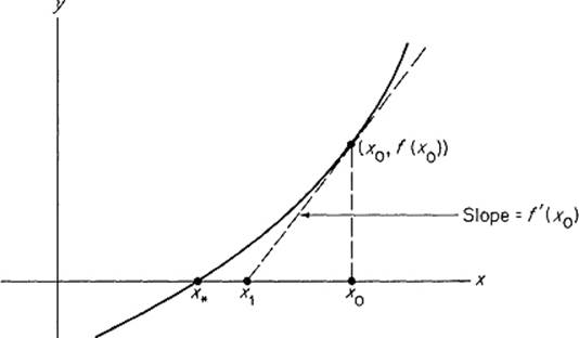
Figure 3.1
Under appropriate hypotheses it can be proved that the sequence ![]() defined inductively by (1) converges to the root x*. We shall not include such a proof here, because our main interest lines in a certain modification of Newton‘s method, rather than in Newton’s method itself.
defined inductively by (1) converges to the root x*. We shall not include such a proof here, because our main interest lines in a certain modification of Newton‘s method, rather than in Newton’s method itself.
In order to avoid the repetitious computation of the derivatives f′(x0), f′(x1), . . . , f′(xn), . . . required in (1), it is tempting to simplify the method by considering instead of (1) the alternative sequence defined inductively by
![]()
But this sequence may fail to converge, as illustrated by Fig. 3.2. However there is a similar simplification which “works”; we consider the sequence ![]() defined inductively by
defined inductively by
![]()
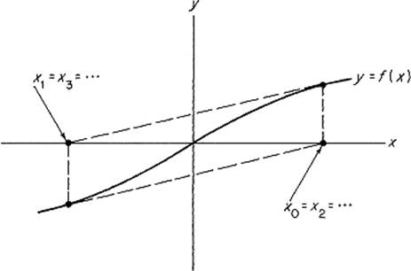
Figure 3.2
where M = max ![]() f′(x)
f′(x)![]() if f′(x) > 0 on [a, b], and M = − max
if f′(x) > 0 on [a, b], and M = − max ![]() f′(x)
f′(x)![]() if f′(x) < 0 on [a, b]. The proof that lim xn = x* if
if f′(x) < 0 on [a, b]. The proof that lim xn = x* if ![]() is defined by (2) makes use of a widely applicable technique which we summarize in the contraction mapping theorem below.
is defined by (2) makes use of a widely applicable technique which we summarize in the contraction mapping theorem below.
The mapping φ: [a, b] → [a, b] is called a contraction mapping with contraction constant k < 1 if
![]()
for all ![]() . The contraction mapping theorem asserts that each contraction mapping has a unique fixed point, that is, a point
. The contraction mapping theorem asserts that each contraction mapping has a unique fixed point, that is, a point ![]() such that φ(x*) = x*, and at the same time provides a sequence of successive approximations to x*.
such that φ(x*) = x*, and at the same time provides a sequence of successive approximations to x*.
Theorem 1.1 Let φ: [a, b] → [a, b] be a contraction mapping with contraction constant k < 1. Then φ has a unique fixed point x*. Moreover, given ![]() , the sequence
, the sequence ![]() defined inductively by
defined inductively by
![]()
converges to x*. In particular,
![]()
for each n.
PROOF Application of condition (3) gives
![]()
so it follows easily by induction that ![]() . From this it follows in turn that, if 0 < n < m, then
. From this it follows in turn that, if 0 < n < m, then
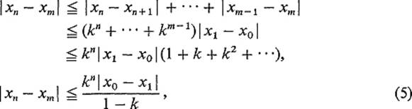
using in the last step the formula for the sum of a geometric series.
Thus the sequence ![]() is a Cauchy sequence, and therefore converges to a point
is a Cauchy sequence, and therefore converges to a point ![]() . Note now that (4) follows directly from (5), letting m → ∞.
. Note now that (4) follows directly from (5), letting m → ∞.
Condition (3) immediately implies that φ is continuous on [a, b], so
![]()
as desired.
Finally, if x** were another fixed point of φ, we would have
![]()
Since k < 1, it follows that x* = x**, so x* is the unique fixed point of φ.
![]()
We are now ready to consider the simplification of Newton's method described by see Eq. (2). Fig. 3.3 for a picture of the sequence defined by this equation.
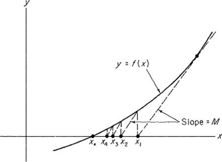
Figure 3.3
Theorem 1.2 Let f: [a, b] → ![]() be a differentiable function with f(a) < 0 < f(b) and
be a differentiable function with f(a) < 0 < f(b) and ![]() for
for ![]() . Given
. Given ![]() , the sequence
, the sequence ![]() defined inductively by
defined inductively by
![]()
converges to the unique root ![]() of the equation f(x) = 0. In particular,
of the equation f(x) = 0. In particular,
![]()
for each n.
PROOF Define φ: [a, b] → ![]() by φ(x) = x − [f(x)/M]. We want to show that φ is a contraction mapping of [a, b]. Since φ′(x) = 1 − [f′(x)/M], we see that
by φ(x) = x − [f(x)/M]. We want to show that φ is a contraction mapping of [a, b]. Since φ′(x) = 1 − [f′(x)/M], we see that
![]()
so φ is a nondecreasing function. Therefore ![]() for all
for all ![]() , because f(a) < 0 < f(b). Thus
, because f(a) < 0 < f(b). Thus ![]() , and φ is a contraction mapping of [a, b].
, and φ is a contraction mapping of [a, b].
Therefore Theorem 1.1 implies that φ has a unique fixed point
![]()
which is clearly the unique root of f(x) = 0, and the sequence ![]() defined by
defined by
![]()
converges to x*. Moreover Eq. (4) gives
![]()
upon substitution of x1 = x0 − [f(x0)/M] and k = 1 − (m/M).
![]()
Roughly speaking, Theorem 1.2 says that, if the point x0 is sufficiently near to a root x* of f(x) = 0 where f′(x*) > 0, then the sequence defined by (2) converges to x*, with M being an upper bound for ![]() f′(x)
f′(x)![]() near x*.
near x*.
Now let us turn the question around. Given a point x* where f(x*) = 0, and a number y close to 0, can we find a point x near x* such that f(x) = y? More generally, supposing that f(a) = b, and that y is close to b, can we find x close to a such that f(x) = y? If so, then
![]()
If f′(a) ≠ 0, we can solve for
![]()
Writing a = x0, the point
![]()
is then a first approximation to a point x such that f(x) = y. This suggests the conjecture that the sequence ![]() defined by
defined by
![]()
converges to a point x such that f(x) = y. In fact we will now prove that the slightly simpler sequence, with f′(xn) replaced by f′(a), converges to the desired point x if y is sufficiently close to b.
Theorem 1.3 Let f: ![]() →
→ ![]() be a
be a ![]() function such that f(a) = b and f′(a) ≠ 0. Then there exist neighborhoods U = [a − δ, a + δ] of a and V = [b − ε, b + ε] of b such that, given
function such that f(a) = b and f′(a) ≠ 0. Then there exist neighborhoods U = [a − δ, a + δ] of a and V = [b − ε, b + ε] of b such that, given ![]() , the sequence
, the sequence ![]() defined inductively by
defined inductively by
![]()
converges to a (unique) point ![]() such that f(x*) = y*.
such that f(x*) = y*.
PROOF Choose δ > 0 so small that
![]()
Then let ![]() . It suffices to show that
. It suffices to show that
![]()
is a contraction mapping of U if ![]() , since φ(x*) = x* clearly implies that f(x*) = y*.
, since φ(x*) = x* clearly implies that f(x*) = y*.
First note that
![]()
if x ∈ U, so φ has contraction constant ![]() . It remains to show that, if
. It remains to show that, if ![]() , then φ maps the interval U into itself. But
, then φ maps the interval U into itself. But
if ![]() and
and ![]() . Thus
. Thus ![]() as desired.
as desired.
![]()
This theorem provides a method for computing local inverse functions by successive approximations. Given y ∈ V, define g(y) to be that point x ∈ U given by the theorem, such that f(x) = y. Then f and g are local inverse functions. If we define a sequence ![]() of functions on V by
of functions on V by
![]()
then we see [by setting xn = gn(y)] that this sequence of functions converges to g.
Example 1 Let f(x) = x2 − 1, a = 1, b = 0. Then (8) gives
Thus it appears that we are generating partial sums of the binomial expansion
![]()
of the inverse function g(y) = (1 + y)1/2.
Next we want to discuss the problem of solving an equation of the form G(x, y) = 0 for y as a function of x. We will say that y = f(x) solves the equation G(x, y) = 0 in a neighborhood of the point (a, b) if G(a, b) = 0 and the graph of f agrees with the zero set of G near (a, b). By the latter we mean that there exists a neighborhood W of (a, b), such that a point (x,y) ∈ W lies on the zero set of G if and only if y = f(x). That is, if (x,y) ∈ W, then G(x, y) = 0 if and only if y = f(x).
Theorem 1.4 below is the implicit function theorem for the simplest case m = n = 1. Consideration of equations such as x2 − y2 = 0 near (0, 0), and x2 + y2 − 1 = 0 near (1, 0), shows that the hypothesis D2 G(a, b) ≠ 0 is necessary.
Theorem 1.4 Let G : ![]() 2 →
2 → ![]() be a
be a ![]() function, and
function, and ![]() a point such that G(a, b) = 0 and D2 G(a, b) ≠ 0. Then there exists a continuous function f : J →
a point such that G(a, b) = 0 and D2 G(a, b) ≠ 0. Then there exists a continuous function f : J → ![]() , defined on a closed interval centered at a, such that y = f(x) solves the equation G(x, y) = 0 in a neighborhood of the point (a, b).
, defined on a closed interval centered at a, such that y = f(x) solves the equation G(x, y) = 0 in a neighborhood of the point (a, b).
In particular, if the functions ![]() are defined inductively by
are defined inductively by
![]()
then the sequence ![]() converges uniformly to f on J.
converges uniformly to f on J.
MOTIVATION Suppose, for example, that D2 G(a, b) > 0. By the continuity of G and D2 G, we can choose a rectangle (see Fig. 3.4) Q = [c1, c2] × [d1, d2] centered at (a, b), such that
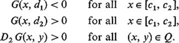
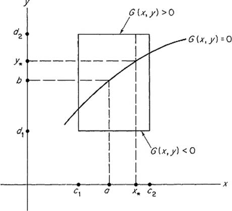
Figure 3.4
Given ![]() , define Gx* : [d1, d2] →
, define Gx* : [d1, d2] → ![]() by
by
![]()
Since Gx*(d1) < 0 < Gx*(d2) and G′x*(y) > 0 on [d1, d2] the intermediate value theorem (see the Appendix) yields a unique point ![]() such that
such that
![]()
Defining f : [c1, c2] → ![]() by f(x*) = y* for each
by f(x*) = y* for each ![]() , we have a function such that y = f(x) solves the equation G(x, y) = 0 in the neighborhood Q of (a, b).
, we have a function such that y = f(x) solves the equation G(x, y) = 0 in the neighborhood Q of (a, b).
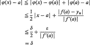
We want to compute y* = f(x*) by successive approximations. By linear approximation we have
![]()
Recalling that G(x*, y*) = 0, and setting y0 = b, this gives
![]()
so
![]()
is our first approximation to y*. Similarly we obtain
![]()
as the (n + 1)th approximation.
What we shall prove is that, if the rectangle Q is sufficiently small, then the slightly simpler sequence ![]() defined inductively by
defined inductively by
![]()
converges to a point y* such that G(x*, y*) = 0.
PROOF First choose ε > 0 such that
![]()
if ![]() and
and ![]() . Then choose δ > 0 less than ε such that
. Then choose δ > 0 less than ε such that
![]()
if ![]() . We will work inside the rectangle W = [a − δ, a + δ] × [b − ε, b + ε], assuming in addition that δ and ε are sufficiently small that
. We will work inside the rectangle W = [a − δ, a + δ] × [b − ε, b + ε], assuming in addition that δ and ε are sufficiently small that ![]() .
.
Let x* be a fixed point of the interval [a − δ, a + δ]. In order to prove that the sequence ![]() defined above converges to a point
defined above converges to a point ![]() with G(x*, y*) = 0, it suffices to show that the function φ : [b − ε, b + ε] →
with G(x*, y*) = 0, it suffices to show that the function φ : [b − ε, b + ε] → ![]() , defined by
, defined by
![]()
is a contraction mapping of the interval [b − ε, b + ε]. First note that
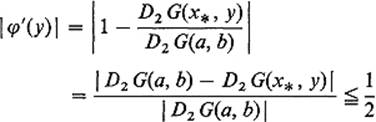
since ![]() . Thus the contraction constant is
. Thus the contraction constant is ![]() .
.
It remains to show that ![]() . But
. But
since ![]() implies
implies ![]() .
.
If we write
![]()
the above argument proves that the sequence ![]() converges to the unique number
converges to the unique number ![]() such that G(x, f(x)) = 0. It remains to prove that this convergence is uniform.
such that G(x, f(x)) = 0. It remains to prove that this convergence is uniform.
To see this, we apply the error estimate of the contraction mapping theorem. Since ![]() because f0(x) = b and
because f0(x) = b and ![]() , and
, and ![]() , we find that
, we find that
![]()
so the convergence is indeed uniform. The functions ![]() are clearly continuous, so this implies that our solution f : [a − δ, a + δ] →
are clearly continuous, so this implies that our solution f : [a − δ, a + δ] → ![]() is also continuous (by Theorem VI.1.2).
is also continuous (by Theorem VI.1.2).
![]()
REMARK We will see later (in Section 3) that the fact that G is ![]() implies that f is
implies that f is ![]() .
.
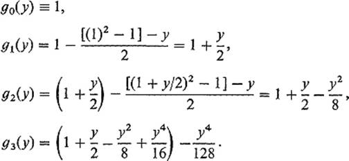
Example 2 Let G(x, y) = x2 + y2 − 1, so G(x, y) = 0 is the unit circle. Let us solve for y = f(x) in a neighborhood of (0, 1) where D2 G(0, 1) = 2. The successive approximations given by (9) are
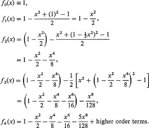
Thus we are generating partial sums of the binomial series
![]()
The preceding discussion is easily generalized to treat the problem of solving an equation of the form
![]()
where G : ![]() m+1 →
m+1 → ![]() for y as a function x = (x1, . . . , xm). Given f :
for y as a function x = (x1, . . . , xm). Given f : ![]() m →
m → ![]() , we say that y = f(x) solves the equation G(x, y) = 0 in a neighborhood of (a, b) if G(a, b) = 0 and the graph of f agrees with the zero set of G near
, we say that y = f(x) solves the equation G(x, y) = 0 in a neighborhood of (a, b) if G(a, b) = 0 and the graph of f agrees with the zero set of G near ![]() .
.
Theorem 1.4 is simply the case m = 1 of the following result.
Theorem 1.5 Let G : ![]() m+1 →
m+1 → ![]() be a
be a ![]() function, and
function, and ![]() a point such that G(a, b) = 0 and Dm+1 G(a, b) ≠ 0. Then there exists a continuous function f : J →
a point such that G(a, b) = 0 and Dm+1 G(a, b) ≠ 0. Then there exists a continuous function f : J → ![]() , defined on a closed cube
, defined on a closed cube ![]() centered at
centered at ![]() , such that y = f(x) solves the equation G(x, y) = 0 in a neighborhood of the point (a, b).
, such that y = f(x) solves the equation G(x, y) = 0 in a neighborhood of the point (a, b).
In particular, if the functions ![]() are defined inductively by
are defined inductively by
![]()
then the sequence ![]() converges uniformly to f on J.
converges uniformly to f on J.
To generalize the proof of Theorem 1.4, simply replace x, a, x* by x, a, x* respectively, and the interval ![]() by the m-dimensional interval
by the m-dimensional interval ![]() .
.
Recall that Theorem 1.5, with the strengthened conclusion that the implicitly defined function f is continuously differentiable (which will be established in Section 3), is all that was needed in Section II.5 to prove that the zero set of a ![]() function G :
function G : ![]() n →
n → ![]() is an (n − 1)-dimensional manifold near each point where the gradient vector ∇G is nonzero. That is, the set
is an (n − 1)-dimensional manifold near each point where the gradient vector ∇G is nonzero. That is, the set
![]()
is an (n − 1)-manifold (Theorem II.5.4).
Exercises
1.1Show that the equation x3 + xy + y3 = 1 can be solved for y = f(x) in a neighborhood of (1, 0).
1.2Show that the set of all points ![]() such that (x + y)5 − xy = 1 is a 1-manifold.
such that (x + y)5 − xy = 1 is a 1-manifold.
1.3Show that the equation y3 + x2y − 2x3 − x + y = 0 defines y as a function of x (for all x). Apply Theorem 1.4 to conclude that y is a continuous function of x.
1.4Let f : ![]() →
→ ![]() and G :
and G : ![]() 2 →
2 → ![]() be
be ![]() functions such that G(x, f(x)) = 0 for all
functions such that G(x, f(x)) = 0 for all ![]() . Apply the chain rule to show that
. Apply the chain rule to show that
![]()
and
![]()
1.5Suppose that G : ![]() m+1 →
m+1 → ![]() is a
is a ![]() function satisfying the hypotheses of Theorem 1.5. Assuming that the implicitly defined function y = f(x1, . . . , xm) is also
function satisfying the hypotheses of Theorem 1.5. Assuming that the implicitly defined function y = f(x1, . . . , xm) is also ![]() , show that
, show that
![]()
1.6Application of Newton's method [Eq. (1)] to the function f(x) = x2 − a, where a > 0, gives the formula ![]() . If
. If ![]() , show that the sequence
, show that the sequence ![]() converges to
converges to ![]() , by proving that
, by proving that ![]() is a contraction mapping of
is a contraction mapping of ![]() . Then calculate
. Then calculate ![]() accurate to three decimal places.
accurate to three decimal places.
1.7Prove that the equation 2 − x − sin x = 0 has a unique real root, and that it lies in the interval [π/6, π/2]. Show that φ(x) = 2 − sin x is a contraction mapping of this interval, and then apply Theorem 1.1 to find the root, accurate to three decimal places.
1.8Show that the equation x + y − z + cos xyz = 0 can be solved for z = f(x, y) in a neighborhood of the origin.
1.9Show that the equation z3 + zex+y + 2 = 0 has a unique solution z = f(x, y) defined for all ![]() . Conclude from Theorem 1.5 that f is continuous everywhere.
. Conclude from Theorem 1.5 that f is continuous everywhere.
1.10If a planet moves along the ellipse x = a cos θ, y = b sin θ, with the sun at the focus ((a2 − b2)1/2, 0), and if t is the time measured from the instant the planet passes through (a, 0), then it follows from Kepler‘s laws that θ and t satisfy Kepler’s equation
![]()
where k is a positive constant and ε = c/a, so ![]() .
.
(a)Show that Kepler's equation can be solved for θ = f(t).
(b)Show that dθ/dt = k/(1 − ε cos θ).
(c)Conclude that dθ/dt is maximal at the “perihelion” (a, 0), and is minimal at the “aphelion” (−a, 0).