Advanced Calculus of Several Variables (1973)

Part I. Euclidean Space and Linear Mappings

Introductory calculus deals mainly with real-valued functions of a single variable, that is, with functions from the real line to itself. Multivariable calculus deals in general, and in a somewhat similar way, with mappings from one Euclidean space to another. However a number of new and interesting phenomena appear, resulting from the rich geometric structure of n-dimensional Euclidean space ⁿ.

In this chapter we discuss ⁿ in some detail, as preparation for the development in subsequent chapters of the calculus of functions of an arbitrary number of variables. This generality will provide more clear-cut formulations of theoretical results, and is also of practical importance for applications. For example, an economist may wish to study a problem in which the variables are the prices, production costs, and demands for a large number of different commodities; a physicist may study a problem in which the variables are the coordinates of a large number of different particles. Thus a “real-life” problem may lead to a high-dimensional mathematical model. Fortunately, modern techniques of automatic computation render feasible the numerical solution of many high-dimensional problems, whose manual solution would require an inordinate amount of tedious computation.

Chapter 1. THE VECTOR SPACE Rⁿ

As a set, ⁿ is simply the collection of all ordered n-tuples of real numbers. That is,

Recalling that the Cartesian product A × B of the sets A and B is by definition the set of all pairs (a, b) such that and , we see that ⁿ can be regarded as the Cartesian product set × · · · × (n times), and this is of course the reason for the symbol ⁿ.

The geometric representation of ³, obtained by identifying the triple (x₁, x₂, x₃) of numbers with that point in space whose coordinates with respect to three fixed, mutually perpendicular “coordinate axes” are x₁, x₂, x₃respectively, is familiar to the reader (although we frequently write (x, y, z) instead of (x₁, x₂, x₃) in three dimensions). By analogy one can imagine a similar geometric representation of ⁿ in terms of n mutually perpendicular coordinate axes in higher dimensions (however there is a valid question as to what “perpendicular” means in this general context; we will deal with this in Section 3).

The elements of ⁿ are frequently referred to as vectors. Thus a vector is simply an n-tuple of real numbers, and not a directed line segment, or equivalence class of them (as sometimes defined in introductory texts).

The set ⁿ is endowed with two algebraic operations, called vector addition and scalar multiplication (numbers are sometimes called scalars for emphasis). Given two vectors x = (x₁, . . . , x_n) and y = (y₁, . . . , y_n) in ⁿ, their sumx + y is defined by

that is, by coordinatewise addition. Given , the scalar multiple ax is defined by

For example, if x = (1, 0, −2, 3) and y = (−2, 1, 4, −5) then x + y = (−1, 1, 2, −2) and 2x = (2, 0, −4, 6). Finally we write 0 = (0, . . . . , 0) and −x = (−1)x, and use x − y as an abbreviation for x + (−y).

The familiar associative, commutative, and distributive laws for the real numbers imply the following basic properties of vector addition and scalar multiplication:

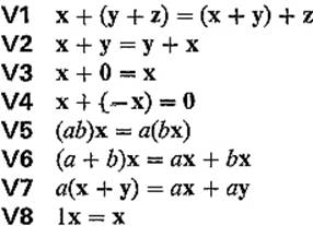
(Here x, y, z are arbitrary vectors in ⁿ, and a and b are real numbers.) V1–V8 are all immediate consequences of our definitions and the properties of . For example, to prove V6, let x = (x₁, . . . , x_n). Then

The remaining verifications are left as exercises for the student.

A vector space is a set V together with two mappings V × V → V and × V → V, called vector addition and scalar multiplication respectively, such that V1–V8 above hold for all and (V3 asserts that there exists such that x + 0 = x for all , and V4 that, given , there exists such that x + (−x) = 0). Thus V1–V8 may be summarized by saying that ⁿ is a vector space. For the most part, all vector spaces that we consider will be either Euclidean spaces, or subspaces of Euclidean spaces.

By a subspace of the vector space V is meant a subset W of V that is itself a vector space (with the same operations). It is clear that the subset W of V is a subspace if and only if it is “closed” under the operations of vector addition and scalar multiplication (that is, the sum of any two vectors in W is again in W, as is any scalar multiple of an element of W)—properties V1–V8 are then inherited by W from V. Equivalently, W is a subspace of V if and only if any linear combination of two vectors in W is also in W (why?). Recall that a linear combination of the vectors v₁, . . . , v_k is a vector of the form a₁ v₁ + · · · + a_k v_k, where the . The span of the vectors is the set S of all linear combinations of them, and it is said that S is generated by the vectors v₁, . . . , v_k.

Example 1ⁿ is a subspace of itself, and is generated by the standard basis vectors

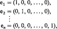
since (x₁, x₂, . . . , x_n) = x₁ e₁ + x₂ e₂ + · · · + x_n e_n. Also the subset of ⁿ consisting of the zero vector alone is a subspace, called the trivial subspace of ⁿ.

Example 2The set of all points in ⁿ with last coordinate zero, that is, the set of all , is a subspace of ⁿ which may be identified with ⁿ⁻¹.

Example 3Given , the set of all such that a₁ x₁ + · · · + a_n x_n = 0 is a subspace of ⁿ (see Exercise 1.1).

Example 4The span S of the vectors is a subspace of ⁿ because, given elements and of S, and real numbers r and s, we have

Lines through the origin in ³ are (essentially by definition) those subspaces of ³ that are generated by a single nonzero vector, while planes through the origin in ³ are those subspaces of ³ that are generated by a pair of non-collinear vectors. We will see in the next section that every subspace V of ⁿ is generated by some finite number, at most n, of vectors; the dimension of the subspace V will be defined to be the minimal number of vectors required to generate V. Subspaces of ⁿ of all dimensions between 0 and n will then generalize lines and planes through the origin in ³.

Example 5If V and W are subspaces of ⁿ, then so is their intersection (the set of all vectors that lie in both V and W). See Exercise 1.2.

Although most of our attention will be confined to subspaces of Euclidean spaces, it is instructive to consider some vector spaces that are not subspaces of Euclidean spaces.

Example 6Let denote the set of all real-valued functions on . If f + g and af are defined by (f + g)(x) = f(x) + g(x) and (af)(x) = af(x), then is a vector space (why?), with the zero vector being the function which is zero for all . If is the set of all continuous functions and is the set of all polynomials, then is a subspace of , and in turn is a subspace of . If _n is the set of all polynomials of degree at most n, then _n is a subspace of which is generated by the polynomials 1, x, x², . . . , xⁿ.

Exercises

1.1Verify Example 3.

1.2Prove that the intersection of two subspaces of ⁿ is also a subspace.

1.3Given subspaces V and W of ⁿ, denote by V + W the set of all vectors v + w with and . Show that V + W is a subspace of ⁿ.

1.4If V is the set of all such that x + 2y = 0 and x + y = 3z, show that V is a subspace of ³.

1.5Let ₀ denote the set of all differentiable real-valued functions on [0, 1] such that f(0) = f(1) = 0. Show that ₀ is a vector space, with addition and multiplication defined as in Example 6. Would this be true if the condition f(0) = f(1) = 0 were replaced by f(0) = 0, f(1) = 1?

1.6Given a set S, denote by (S, ) the set of all real-valued functions on S, that is, all maps S → R. Show that (S, ) is a vector space with the operations defined in Example 6. Note that ({1, . . . , n}, ) can be interpreted as ⁿ since the function may be regarded as the n-tuple (φ(1), φ(2), . . . , φ(n)).