Advanced Calculus of Several Variables (1973)

Part III. Successive Approximations and Implicit Functions

Chapter 4. MANIFOLDS IN Rⁿ

We continue here the discussion of manifolds that was begun in Section II.5. Recall that a k-dimensional manifold in ⁿ is a set M that looks locally like the graph of a mapping from ^k to ^n−k. That is, every point of M lies in an open subset V of ⁿ such that is a k-dimensional patch. Recall that this means there exists a permutation of x₁, . . . , x_n, and a differentiable mapping h : U → ^n−k defined on an open set , such that

see Fig. 3.9. We will call P a or smooth patch if the mapping h is . The manifold M will be called or smooth if it is a union of smooth patches.

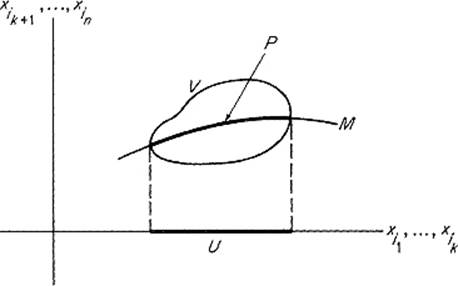
Figure 3.9

There are essentially three ways that a k-manifold in ⁿ can appear (locally):

(a)as the graph of a mapping ^k → ^n−k,

(b)as the zero set of a mapping ⁿ → ^n−k,

(c)as the image of a mapping ^k → ⁿ.

The definition of a manifold is based on (a), which is actually a special case of both (b) and (c), since the graph of f: ^k → ^n−k is the same as the zero set of G(x, y) = f(x) − y, and is also the image of F : ^k → ⁿ, where F(x) = (x, f(x)). We want to give conditions under which (b) and (c) are, in fact, equivalent to (a).

Recall that our study of the Lagrange multiplier method in Section II.5 was based on the appearance of manifolds in guise (b). The following result was stated (without proof) in Theorem II.5.7.

Theorem 4.1 Let G : ⁿ → ^m be a mapping, where k = n − m > 0. If M is the set of all those points for which the derivative matrix G′(x) has rank m, then M is a smooth k-manifold.

PROOF We need to show that each point p of M lies in a smooth k-dimensional patch on M. By Theorem I.5.4, the fact, that the rank of the m × n matrix G′(p) is m, implies that some m of its column vectors are linearly independent. The column vectors of the matrix G′ are simply the partial derivative vectors ∂G/∂x₁, . . . , ∂G/∂x_n, and let us suppose we have rearranged the coordinates in ⁿ so that it is the last m of these partial derivative vectors that are linearly independent. If we write

where , then it follows that the partial derivative matrix D₂G(p) is nonsingular.

Consequently the implicit mapping theorem applies to provide us with a neighborhood V of p = (a, b) in ⁿ, a neighborhood U of a in ^k, and a mapping f : U → ^m such that y = f(x) solves the equation G(x, y) = 0 in V. Clearly the graph of f is the desired smooth k-dimensional patch.

Thus conditions (a) and (b) are equivalent, subject to the rank hypothesis in Theorem 4.1.

When we study integration on manifolds in Chapter V, condition (c) will be the most important of the three. If M is a k-manifold in ⁿ, and U is an open subset of ^k, then a one-to-one mapping φ : U → M can be regarded as a parametrization of the subset φ(U) of M. For example, the student is probably familiar with the spherical coordinates parametrization of the unit sphere , defined by

The theorem below asserts that, if the subset M of ⁿ can be suitably parametrized by means of mappings from open subsets of ^k to M, then M is a smooth k-manifold.

Let φ : U → ⁿ be a mapping defined on an open subset U of . Then we call φ regular if the derivative matrix φ′(u) has maximal rank k, for each u ∈ U. According to the following theorem, a subset M of ⁿ is a smooth k-manifold if it is locally the image of a regular mapping defined on an open subset of ^k.

Theorem 4.2 Let M be a subset of ⁿ. Suppose that, given p ∈ M, there exists an open set and a regular mapping φ : U → ⁿ such that , with φ(U′) being an open subset of M for each open set . Then M is a smooth k-manifold.

The statement that φ(U′) is an open subset of M means that there exists an open set W′ in ⁿ such that . The hypothesis that φ(U′) is open in M, for every open subset U′ of U, and not just for U itself, is necessary if the conclusion that M is a k-manifold is to follow. That this is true may be seen by considering a figure six in the plane—although it is not a 1-manifold (why?); there obviously exists a one-to-one regular mapping φ : (0, 1) → ² that traces out the figure six.

PROOF Given p ∈ M and φ : U → M as in the statement of the theorem, we want to show that p has a neighborhood (in ⁿ) whose intersection with M is a smooth k-dimensional patch. If φ(a) = p, then the n × k matrix φ′(a) has rank k. After relabeling coordinates in ⁿ if necessary, we may assume that the k × k submatrix consisting of the first k rows of φ′(a) is nonsingular.

Write p = (b, c) with and , and let π : ⁿ → ^k denote the projection onto the first k coordinates,

If f : U → ^k is defined by

then f(a) = b, and the derivative matrix f′(a) is nonsingular, being simply the k × k submatrix of φ′(a) referred to above.

Consequently the inverse mapping theorem applies to give neighborhoods U′ of a and V′ of b such that f : U′ → V′ is one-to-one, and the inverse g : V′ → U′ is . Now define h : V′ → ^n−k by

Since the graph of h is P = φ(U′), and there exists (by hypothesis) an open set W′ in ⁿ with , we see that p lies in a smooth k-dimensional patch on M, as desired.

REMARK Note that, in the above notation, the mapping

is a local inverse to φ. That is, Φ is a mapping on the open subset W′ of ⁿ, and Φ(x) = φ⁻¹(x) for . This fact will be used in the proof of Theorem 4.3 below.

If M is a smooth k-manifold, and φ : U → M satisfies the hypotheses of Theorem 4.2, then the mapping φ is called a coordinate patch for M provided that it is one-to-one. That is, a coordinate patch for M is a one-to-one regular mapping φ : U → ⁿ defined on an open subset of ^k, such that φ(U′) is an open subset of M, for each open subset U′ of U.

Note that the “local graph” patches, on which we based the definition of a manifold, yield coordinate patches as follows. If M is a smooth k-manifold in ⁿ, and W is an open set such that is the graph of the mapping , then the mapping φ : U → ⁿ defined by φ(u) = (u, f(u)) is a coordinate patch for M. We leave it as exercise for the reader to verify this fact. At any rate, every smooth manifold M possesses an abundance of coordinate patches. In particular, every point of M lies in the image of some coordinate patch, so there exists a collection of coordinate patches for M such that

U_α being the domain of definition of φ_α. Such a collection of coordinate patches is called an atlas for M.

The most important fact about coordinate patches is that they overlap differentiably, in the sense of the following theorem (see Fig. 3.10).

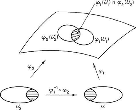
Figure 3.10

Theorem 4.3 Let M be a smooth k-manifold in ⁿ, and let φ₁ : U₁ → M and φ₂ : U₂ → M be two coordinate patches with non-empty. Then the mapping

is continuously differentiable.

PROOF Given , the remark following the proof of Theorem 4.2 provides a local inverse Φ to φ₁, defined on a neighborhood of p in ⁿ. Then agrees, in a neighborhood of the point , with the composition Φ φ₂ of two mappings.

Now let be an atlas for the smooth k-manifold , and write

if is nonempty. Then T_ij is a mapping by the above theorem, and has the inverse T_ji. It follows from the chain rule that

so det T′_ij(x) ≠ 0 wherever T_ij is defined.

The smooth k-manifold M is called orientable if there exists an atlas {φ_i} for M such that each of the “change of coordinates” mappings T_ij defined above has positive Jacobian determinant,

wherever it is defined. The pair (M, {φ_i}) is then called an oriented k-manifold.

Not every manifold can be oriented. The classical example of a nonorientable manifold is the Möbius strip, a model of which can be made by gluing together the ends of a strip of paper after given it a half twist. We will see the importance of orientability when we study integration on manifolds in Chapter V.

Exercises

4.1Let φ : U → ⁿ and ψ : V → ⁿ be two coordinate patches for the smooth k-manifold M. Say that φ and ψ overlap positively (respectively negatively) if det(φ⁻¹ ψ)′ is positive (respectively negative) wherever defined. Now define ρ : ^k → ^k by

If φ and ψ overlap negatively, and = ψ ρ : ρ⁻¹(V) → ⁿ, prove that the coordinate neighborhoods φ and overlap positively.

4.2Show that the unit sphere Sⁿ⁻¹ has an atlas consisting of just two coordinate patches. Conclude from the preceding exercise that Sⁿ⁻¹ is orientable.

4.3Let M be a smooth k-manifold in ⁿ. Given p ∈ M, show that there exists an open subset W of ⁿ with p ∈ W, and a one-to-one mapping f: W → ⁿ, such that is an open subset of .

4.4Let M be a smooth k-manifold in ⁿ, and N a smooth (k − 1)-manifold with . If φ : U → M is a coordinate patch such that is nonempty, show that is a smooth (k − 1)-manifold in ^k. Conclude from the preceding exercise that, given p ∈ N, there exists a coordinate patch ψ : V → M with , such that is an open subset of .

4.5If U is an open subset of , and φ : U → ³ is a mapping, show that φ is regular if and only if ∂φ/∂u × ∂φ/∂v ≠ 0 at each point of U. Conclude that φ is regular if and only if, at each point of U, at least one of the three Jacobian determinants

is nonzero.

4.6The 2-manifold M in ³ is called two-sided if there exists a continuous mapping n : M → ³ such that, for each x ∈ M, the vector n(x) is perpendicular to the tangent plane T_x to M at x. Show that M is two-sided if it is orientable. Hint: If φ : U → ³ is a coordinate patch for M, then ∂φ/∂u(u) × ∂φ/∂v(u) is perpendicular to T_φ(u). If φ : U → ³ and ψ : V → ³ are two coordinate patches for M that overlap positively, and u ∈ U and v ∈ V are points such that , show that the vectors

are positive multiples of each other.