Advanced Calculus of Several Variables (1973)

Part IV. Multiple Integrals

Chapters II and III were devoted to multivariable differential calculus. We turn now to a study of multivariable integral calculus.

The basic problem which motivates the theory of integration is that of calculating the volumes of sets in ⁿ. In particular, the integral of a continuous nonnegative, real-valued function f on an appropriate set is supposed to equal the volume of the region in ⁿ⁺¹ that lies over the set S and under the graph of f. Experience and intuition therefore suggest that a thorough discussion of multiple integrals will involve the definition of a function which associates with each “appropriate” set a nonnegative real number v(A) called its volume, satisfying the following conditions (in which A and B are subsets of ⁿ whose volume is defined):

(a)If , then .

(b)If A and B are nonoverlapping sets (meaning that their interiors are disjoint), then .

(c)If A and B are congruent sets (meaning that one can be carried onto the other by a rigid motion of ⁿ), then v(A) = v(B).

(d)If I is a closed interval in ⁿ, that is, I = I₁ × I₂ × · · · × I_n where , then v(I) = (b₁ − a₁)(b₂ − a₂) · · · (b_n − a_n).

Conditions (a)–(d) are simply the natural properties that should follow from any reasonable definition of volume, if it is to agree with one's intuitive notion of “size” for subsets of ⁿ.

In Section 1 we discuss the concept of volume, or “area,” for subsets of the plane ², and apply it to the 1-dimensional integral. This will serve both as a review of introductory integral calculus, and as motivation for the treatment in Sections 2 and 3 of volume and the integral in ⁿ. Subsequent sections of the chapter are devoted to iterated integrals, change of variables in multiple integrals, and improper integrals.

Chapter 1. AREA AND THE 1-DIMENSIONAL INTEGRAL

The Greeks attempted to determine areas by what is called the “method of exhaustion.” Their basic idea was as follows: Given a set A whose area is to be determined, we inscribe in it a polygonal region whose area can easily be calculated (by breaking it up into nonoverlapping triangles, for instance). This should give an underestimate to the area of A. We then choose another polygonal region which more nearly fills up the set A, and therefore gives a better approximation to its area (Fig. 4.1). Continuing this process, we attempt to “exhaust”

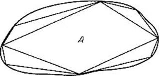
Figure 4.1

the set A with an increasing sequence of inscribed polygons, whose areas should converge to the area of the set A.

However, before attempting to determine or to measure area, we should say precisely what it is that we seek to determine. That is, we should start with a definition of area. The following definition is based on the idea of approximating both from within and from without, but using collections of rectangles instead of polygons. We start by defining the area a(R) of a rectangle R to be the product of the lengths of its base and height. Then, given a bounded set S in the plane ², we say that its area is α if and only if, given ε > 0, there exist both

(1)a finite collection R₁′, . . . , R_k′ of nonoverlapping rectangles, each contained in S, with (Fig. 4.2a),

and

(2)A finite collection R₁″, . . . , R_l″ of rectangles which together contain S, with (Fig. 4.2b).

If there exists no such number α, then we say that the set S does not have area, or that its area is not defined.

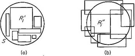
Figure 4.2

Example 1Not every set has area. For instance, if

then S contains no (nondegenerate) rectangle. Hence and for any two collections as above (why?). Thus no number α satisfies the definition (why?).

Example 2We verify that the area of a triangle of base b and height a is . First subdivide the base [0, b] into n equal subintervals, each of length b/n. See Fig. 4.3. Let R_k′ denote the rectangle with height (k − 1)a/n and base [(k− 1)b/n, kb/n], and R_k″ the rectangle with base [(k − 1)b/n, kb/n] and height ka/n. Then the sum of the areas of the inscribed rectangles is

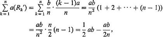
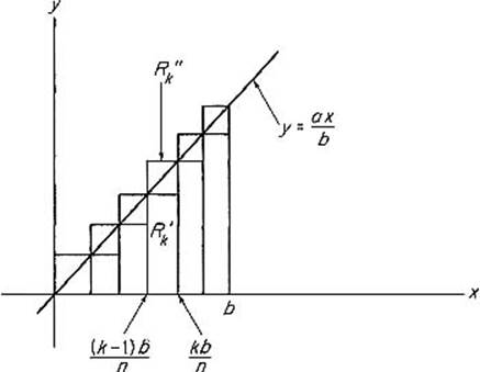
Figure 4.3

while the sum of the areas of the circumscribed rectangles is

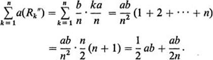
Hence let . Then, given ε > 0, we can satisfy conditions (1) and (2) of the definition by choosing n so large that ab/2n < ε.

We can regard area as a nonnegative valued function a : → , where is the collection of all those subsets of ² which have area. We shall defer a systematic study of area until Section 2, where Properties A–E below will be verified. In the remainder of this section, we will employ these properties of area to develop the theory of the integral of a continuous function of one variable.

AIf S and T have area and , then (see Exercise 1.3 below).

BIf S and T are two nonoverlapping sets which have area, then so does , and .

CIf S and T are two congruent sets and S has area, then so does T, and a(S) = a(T).

DIf R is a rectangle, then a(R) = the product of its base and height (obvious from the definition).

EIf where f is a continuous nonnegative function on [a, b], then S has area.

We now define the integral of a continuous function f: [a, b] → . Suppose first that f is nonnegative on [a, b], and consider the “ordinate set”

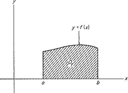
Figure 4.4

pictured in Fig. 4.4. Property E simply says that has area. We define the integral of the nonnegative continuous function f: [a, b] → by

the area of its ordinate set. Notice that, if on [a, b], then

by Properties A and D (see Fig. 4.5a), while

if by property B (see Fig. 4.5b).

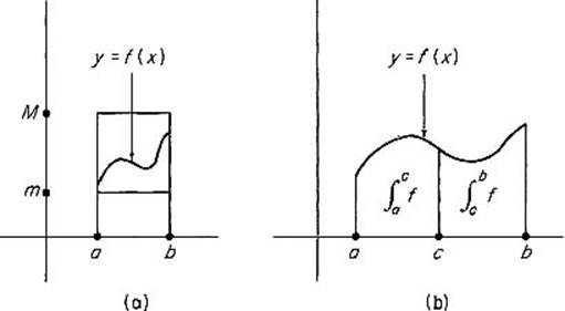
Figure 4.5

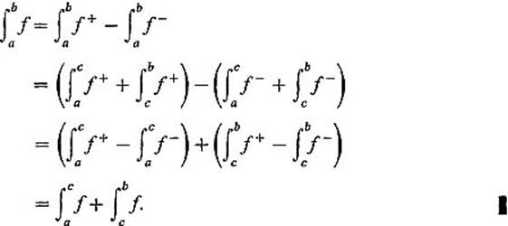
If f is an arbitrary continuous function on [a, b], we consider its positive and negative parts f⁺ and f⁻, defined on [a, b] by

and

Notice that f = f⁺ − f⁻, and that f⁺ and f⁻ are both nonnegative functions. Also the continuity of f implies that of f⁺ and f⁻ (Exercise 1.4). We can therefore define the integral of f on [a, b] by

In short, is “the area above the x-axis minus the area below the x-axis” (see Fig. 4.6). We first verify that (1) and (2) above hold for arbitrary continuous functions.

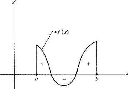
Figure 4.6

Lemma 1.1If , then

PROOFThis is true for f because it is true for both f⁺ and f⁻:

Lemma 1.2If on [a, b], then

PROOFWe shall show that the proof that is similar and is left as an exercise.

Suppose first that M > 0. Then

because on [a, b], so that is contained in the rectangle with base [a, b] and height M (Fig. 4.7).

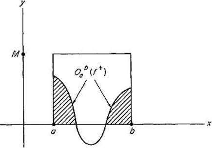
Figure 4.7

If , then , so f⁺(x) = 0, f⁻(x) = −f(x) on [a, b], and . Hence

because contains the rectangle of height −M.

Lemmas 1.1 and 1.2 provide the only properties of the integral that are needed to prove the fundamental theorem of calculus.

Theorem 1.3If f : [a, b] → is continuous, and F: [a, b] → is defined by , then F is differentiable, with F′ = f.

PROOFDenote by m(h) and M(h) the minimum and maximum values respectively of f on [x, x + h]. Then

by Lemma 1.1, and

by Lemma 1.2, so

Since lim_h→0 m(h) = lim_h→0 M(h) = f(x) because f is continuous at x, it follows from (3) that

as desired.

The usual method of computing integrals follows immediately from the fundamental theorem.

Corollary 1.4If f is continuous and G′ = f on [a, b], then

PROOFIf on [a, b], then

by the fundamental theorem. Hence

Now , so

It also follows quickly from the fundamental theorem that integration is a linear operation.

Theorem 1.5If the functions f and g are continuous on [a, b], and , then

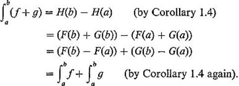
PROOFLet F and G be antiderivatives of f and g, respectively (provided by the fundamental theorem), and let H = F + G on [a, b]. Then H′ = (F + G)′ = F′ + G′ = f + g, so

The proof that is similar.

Theorem 1.6If on [a, b], then

PROOFSince , Theorem 1.5 and Lemma 1.2 immediately give

Applying Theorem 1.6 with g = f, we see that

if on [a, b].

It is often convenient to write

and we do this in the following two familiar theorems on techniques of integration.

Theorem 1.7(Substitution) Let f have a continuous derivative on [a, b], and let g be continuous on [c, d], where . Then

PROOFLet G be an antiderivative of g on [c, d]. Then

by the chain rule, so

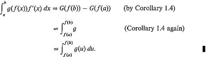
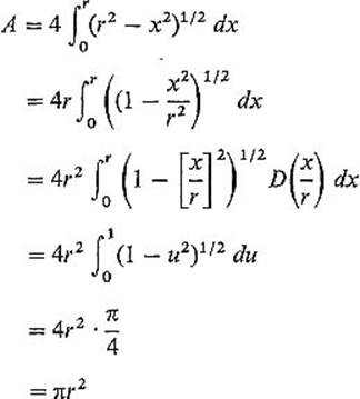
Example 3Using the substitution rule, we can give a quick proof that the area of a circle of radius r is indeed A = πr². Since π is by definition the area of the unit circle, we have (see Fig. 4.8)

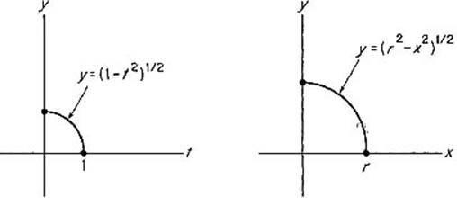
Figure 4.8

Then

Theorem 1.8(Integration by Parts) If f and g are continuously differentiable on [a, b], then

PROOF

or

so

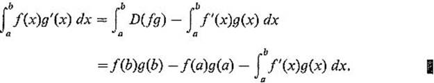
The integration by parts formula takes the familiar and memorable form

if we write u = f(x), v = g(x), and further agree to the notation du = f′(x) dx, dv = g′(x) dx in the integrands.

Exercises

1.1Calculate the area under y = x² over the interval [0, 1] by making direct use of the definition of area.

1.2Apply the fundamental theorem to calculate the area in the previous exercise.

1.3Prove Property A of area. Hint: Given , suppose to the contrary that a(T) < a(S), and let . Show that you have a contradiction, assuming (as you may) that, if the rectangles R₁″, . . . , R_m″ together contain the rectangles R₁′, . . . , R_n′, then .

1.4Prove that the positive and negative parts of a continuous function are continuous.

1.5If f is continuous on [a, b], and

prove that G′(x) = −f(x) on [a, b]. (See the proof of the fundamental theorem.)

1.6Prove the other part of Theorem 1.5, that is, that if c is a constant.

1.7Use integration by parts to establish the “reduction formula”

In particular, .

1.8Use the formula in Exercise 1.7 to show by mathematical induction that

and

1.9(a)Conclude from the previous exercise that

(b)Use the inequality

and the first formula in Exercise 1.8 to show that

(c)Conclude from (a) and (b) that

This result is usually written as an “infinite product,” known as Wallis' product:

1.10Deduce from Wallis' product that

Hint: Multiply and divide the right-hand side of

by 2 · 2 · 4 · 4 · · · · · (2n) · (2n). This yields

1.11Write for each n, thereby defining the sequence . Assuming that lim_{n → ∞} a_n = a ≠ 0, deduce from the previous problem that a = (2π)^1/2. Hence n! and (2πn)^1/2(n/e)ⁿ are asymptotic as n → ∞,

meaning that the limit of their ratio is 1. This is a weak form of “Stirling's formula.”