Advanced Calculus of Several Variables (1973)
Part IV. Multiple Integrals
Chapter 3. STEP FUNCTIONS AND RIEMANN SUMS
As a tool for studying the integral, we introduce in this section a class of very simple functions called step functions. We shall see first that the properties of step functions are easily established, and then that an arbitrary function is integrable if and only if it is, in a certain precise sense, closely approximated by step functions.
The function h : ![]() n →
n → ![]() is called a step function if and only if h can be written as a linear combination of characteristic functions φ1, . . . , φp of intervals I1, . . . , Ip whose interiors are mutually disjoint, that is,
is called a step function if and only if h can be written as a linear combination of characteristic functions φ1, . . . , φp of intervals I1, . . . , Ip whose interiors are mutually disjoint, that is,
![]()
with coefficients ![]() . Here the intervals I1, I2·, . . . , Ip are not necessarily closed—each is simply a product of intervals in
. Here the intervals I1, I2·, . . . , Ip are not necessarily closed—each is simply a product of intervals in ![]() (the latter may be either open or closed or “half-open”).
(the latter may be either open or closed or “half-open”).
Theorem 3.1If h is a step function, ![]() as above, then h is integrable with
as above, then h is integrable with
![]()
PROOFIn fact h is admissible, since it is clearly continuous except possibly at the points of the negligible set ![]() .
.
Assume for simplicity that each ai > 0. Then the ordinate set Oh contains the set
![]()
whose volume is clearly ![]() , and is contained in the union of A and the negligible set
, and is contained in the union of A and the negligible set
![]()
It follows easily that
![]()
It follows immediately from Theorem 3.1 that, if h is a step function and ![]() , then ∫ ch = c ∫ h. The following theorem gives the other half of the linearity of the integral on step functions.
, then ∫ ch = c ∫ h. The following theorem gives the other half of the linearity of the integral on step functions.
Theorem 3.2If h and k are step functions, then so is h + k, and ∫(h + k) = ∫ h + ∫ k.
PROOFIn order to make clear the idea of the proof, it will suffice to consider the simple special case
![]()
where φ and ψ are the characteristic functions of intervals I and J. If I and J have disjoint interiors, then the desired result follows from the previous theorem.
Otherwise ![]() is an interval I0, and it is easily seen that I − I0 and J − I0 are disjoint unions of intervals (Fig. 4.14)
is an interval I0, and it is easily seen that I − I0 and J − I0 are disjoint unions of intervals (Fig. 4.14)
![]()
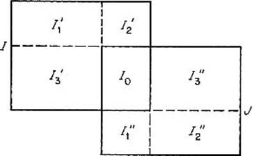
Figure 4.14
Then
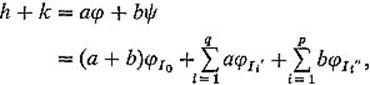
so we have expressed h + k as a step function. Theorem 3.1 now gives
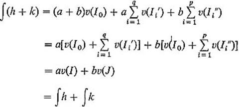
as desired. The proof for general step functions h and k follows from this construction by induction on the number of intervals involved.
![]()
Our main reason for interest in step functions lies in the following characterization of integrable functions.
Theorem 3.3Let f : ![]() n →
n → ![]() be a bounded function with bounded support. Then f is integrable if and only if, given ε > 0, there exist step functions h and k such that
be a bounded function with bounded support. Then f is integrable if and only if, given ε > 0, there exist step functions h and k such that
![]()
in which case ![]() .
.
PROOFSuppose first that, given ε > 0, step functions h and k exist as prescribed. Then the set
![]()
has volume equal to ∫(k − h) < ε. But S contains the set ![]() f = ∂Of −
f = ∂Of − ![]() n (Fig. 4.15). Thus for every ε > 0,
n (Fig. 4.15). Thus for every ε > 0, ![]() f lies in a set of volume < ε. It follows easily that
f lies in a set of volume < ε. It follows easily that ![]() f is a negligible set. If Q is a rectangle in
f is a negligible set. If Q is a rectangle in ![]() n such that f = 0 outside Q, then
n such that f = 0 outside Q, then ![]() and
and ![]() are both subsets of
are both subsets of ![]() , so it follows that both are negligible. Therefore the ordinate sets
, so it follows that both are negligible. Therefore the ordinate sets ![]() and
and ![]() are both contented, so f is integrable. The fact that
are both contented, so f is integrable. The fact that ![]() follows from Exercise 2.6 (without using Axioms I and II, which we have not yet proved).
follows from Exercise 2.6 (without using Axioms I and II, which we have not yet proved).
Now suppose that f is integrable. Since this implies that both f+ and f− are integrable, we may assume without loss that ![]() . Then the fact that f is integrable means by definition that Of is contented. Hence, given ε > 0, there exist
. Then the fact that f is integrable means by definition that Of is contented. Hence, given ε > 0, there exist
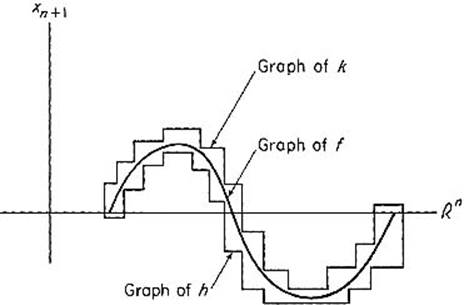
Figure 4.15
nonoverlapping intervals I1, . . . , Iq contained in Of, and intervals J1, . . . , Jp with ![]() , such that
, such that
![]()
see Fig. 4.16.
Given ![]() , define
, define
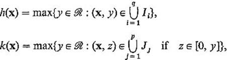
if the vertical line in ![]() n+1 through
n+1 through ![]() intersects some Ii (respectively, some Jj), and let h(x) = 0 (respectively, k(x) = 0) otherwise. Then h and k are step
intersects some Ii (respectively, some Jj), and let h(x) = 0 (respectively, k(x) = 0) otherwise. Then h and k are step
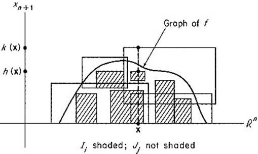
Figure 4.16
functions such that ![]() . Since
. Since
![]()
the above inequalities imply that
as desired.
![]()
ExampleWe can apply Theorem 3.3 to prove again that continuous functions are integrable. Let f : ![]() n →
n → ![]() be a continuous function having compact support. Since it follows that the nonnegative functions f+ and f− are continuous, we may as well assume that f itself is nonnegative. Let
be a continuous function having compact support. Since it follows that the nonnegative functions f+ and f− are continuous, we may as well assume that f itself is nonnegative. Let ![]() be a closed interval such that f = 0 outside Q. Then f is uniformly continuous on Q (by Theorem 8.9 of Chapter I) so, given ε > 0, there exists δ > 0 such that
be a closed interval such that f = 0 outside Q. Then f is uniformly continuous on Q (by Theorem 8.9 of Chapter I) so, given ε > 0, there exists δ > 0 such that
![]()
Now let ![]() = {Q1, . . . , Ql} be a partition of Q into nonoverlapping closed intervals, each of diameter less than δ. If
= {Q1, . . . , Ql} be a partition of Q into nonoverlapping closed intervals, each of diameter less than δ. If
and ![]() then
then ![]() and
and
![]()
so Theorem 3.3 applies.
We are now prepared to verify Axioms I and II of the previous section. Given integrable functions f1 and f2, and real numbers a1 and a2, we want to prove that a1f1 + a2f2 is integrable with
![]()
We suppose for simplicity that a1 > 0, a2 > 0, the proof being similar in the other cases.
Given ε > 0, Theorem 3.3 provides step functions h1, h2, k1, k2 such that
![]()
and ∫(ki − hi) < ε/2ai for i = 1, 2. Then
![]()
where h and k are step functions such that
![]()
So it follows from Theorem 3.3 that a1f1 + a2f2 is integrable.
At the same time it follows from (1) that
![]()
(by Exercise 2.6), and similarly from (2) that
![]()
Since ∫ k − ∫ h < ε, it follows that ∫(a1f1 + a2f2) and a1 ∫f1 + a2∫f2 differ by less than ε. This being true for every ε > 0, we conclude that
![]()
We now relate our definition of the integral to the “Riemann sum” definition of the single-variable integral which the student may have seen in introductory calculus. The motivation for this latter approach is as follows. Let f : [a, b] → ![]() be a nonnegative function. Let the points a = x0 < x1 < · · · < xk = b subdivide the interval [a, b] into k subintervals [x0, x1], [x1, x2], . . . , [xk−1, xk]. For each i = 1, . . . , k, choose a point
be a nonnegative function. Let the points a = x0 < x1 < · · · < xk = b subdivide the interval [a, b] into k subintervals [x0, x1], [x1, x2], . . . , [xk−1, xk]. For each i = 1, . . . , k, choose a point ![]() . (Fig. 4.17). Then f(xi*)(xi − xi−1) is the area of the rectangle of height f(xi*) whose base is the ith subinterval [xi−1, xi], so one suspects that the sum
. (Fig. 4.17). Then f(xi*)(xi − xi−1) is the area of the rectangle of height f(xi*) whose base is the ith subinterval [xi−1, xi], so one suspects that the sum
![]()
should be a “good approximation” to the area of Of if the subintervals are sufficiently small. Notice that the Riemann sum R is simply the integral of the step function
![]()
where φi denotes the characteristic function of the interval [xi−1, xi].
Recall that a partition of the interval Q is a collection ![]() = {Q1, . . . , Qk} of closed intervals, with disjoint interiors, such that
= {Q1, . . . , Qk} of closed intervals, with disjoint interiors, such that ![]() . By the mesh of
. By the mesh of ![]()
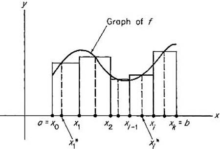
Figure 4.17
is meant the maximum of the diameters of the Qi. A selection for ![]() is a set
is a set ![]() = {x1, . . . , xk} of points such that
= {x1, . . . , xk} of points such that ![]() for each i. If f :
for each i. If f : ![]() n →
n → ![]() is afunction such that f = 0 outside of Q, then the Riemann sum for f corresponding to the partition
is afunction such that f = 0 outside of Q, then the Riemann sum for f corresponding to the partition ![]() and selection
and selection ![]() is
is
![]()
Notice that, by Theorem 3.1, the Riemann sum R(f, ![]() ,
, ![]() ) is simply the integral of the step function
) is simply the integral of the step function
![]()
where φi denotes the characteristic function of Qi.
Theorem 3.4Suppose f : ![]() n →
n → ![]() is bounded and vanishes outside the interval Q. Then f is integrable with ∫f = I if and only if, given ε > 0, there exists δ > 0 such that
is bounded and vanishes outside the interval Q. Then f is integrable with ∫f = I if and only if, given ε > 0, there exists δ > 0 such that
![]()
whenever ![]() is a partition of Q with mesh <δ and
is a partition of Q with mesh <δ and ![]() is a selection for
is a selection for ![]() .
.
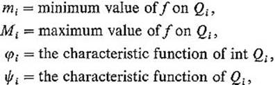
PROOFIf f is integrable, choose M > 0 such that ![]() for all x. By Theorem 3.3 there exist step functions h and k such that
for all x. By Theorem 3.3 there exist step functions h and k such that ![]() and ∫ (k − h) < ε/2. By the construction of the proof of Theorem 3.2, we may assume that h and k are linear combinations of the characteristic functions of intervals whose closures are the same. That is, there is a partition
and ∫ (k − h) < ε/2. By the construction of the proof of Theorem 3.2, we may assume that h and k are linear combinations of the characteristic functions of intervals whose closures are the same. That is, there is a partition ![]() 0 = {Q1, . . . , Qs} of Q such that
0 = {Q1, . . . , Qs} of Q such that
![]()
where Qi is the closure of the interval of which φi is the characteristic function, and likewise for ψi.
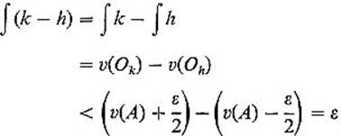
Now let ![]() int Qi. Then v(A) = 0, so there exists δ > 0 such that, if
int Qi. Then v(A) = 0, so there exists δ > 0 such that, if ![]() is a partition of Q with mesh <δ, then the sum of the volumes of those intervals P1, . . . , Pk of
is a partition of Q with mesh <δ, then the sum of the volumes of those intervals P1, . . . , Pk of ![]() which intersect A is less than ε/4M. Let Pk+1, . . . , Pl be the remaining intervals of
which intersect A is less than ε/4M. Let Pk+1, . . . , Pl be the remaining intervals of ![]() , that is, those which lie interior to the Qi.
, that is, those which lie interior to the Qi.
If ![]() = {x1, . . . , xl} is a selection for
= {x1, . . . , xl} is a selection for ![]() , then
, then ![]() if i = k + 1, . . . , l, so that
if i = k + 1, . . . , l, so that
![]()
are both between ![]() and
and ![]() so it follows that
so it follows that
![]()
because ∫Q(k − h) < ε/2 by assumption.
Since ![]() for all x, both
for all x, both
![]()
lie between ![]() and
and ![]() , so it follows that
, so it follows that
![]()
Since ![]() , (3) and (4) finally imply by the triangle inequality that
, (3) and (4) finally imply by the triangle inequality that ![]() I − R(f,
I − R(f, ![]() ,
, ![]() )
)![]() < ε as desired.
< ε as desired.
Conversely, suppose ![]() = {P1, . . . , Pp} is a partition of Q such that, given any selection
= {P1, . . . , Pp} is a partition of Q such that, given any selection ![]() for
for ![]() , we have
, we have
![]()
Let Q1, . . . , Qp be disjoint intervals (not closed) such that ![]() i = Pi, i = 1, . . . , p, and denote by φi the characteristic function of Qi. If
i = Pi, i = 1, . . . , p, and denote by φi the characteristic function of Qi. If
![]()
then
![]()
are step functions such that ![]() .
.
Choose selections ![]() ′ = {x1′, . . . , xp′} and
′ = {x1′, . . . , xp′} and ![]() ″ = {x1″, . . . , xp″} for
″ = {x1″, . . . , xp″} for ![]() such that
such that
![]()
for each i. Then
and similarly
![]()
Then
so it follows from Theorem 3.3 that f is integrable.
![]()
Theorem 3.4 makes it clear that the operation of integration is a limit process. This is even more apparent in Exercise 3.2, which asserts that, if f : ![]() n →
n → ![]() is an integrable function which vanishes outside the interval Q, and
is an integrable function which vanishes outside the interval Q, and ![]() is a sequence of partitions of Q with associated selections
is a sequence of partitions of Q with associated selections ![]() such that limk→∞ (mesh of
such that limk→∞ (mesh of ![]() k) = 0, then
k) = 0, then
![]()
This observation leads to the formulation of several natural and important integration questions as interchange of limit operations questions.
(1)Let ![]() and
and ![]() be contented sets, and f : A × B →
be contented sets, and f : A × B → ![]() a continuous function. Define g : A →
a continuous function. Define g : A → ![]() by
by
![]()
where fx(y) = f(x, y). Is g continuous on A? This is the question as to whether
![]()
for each ![]() . According to Exercise 3.3, this is true if f is uniformly continuous.
. According to Exercise 3.3, this is true if f is uniformly continuous.
(2)Let ![]() be a sequence of integrable functions on the contented set A, which converges (pointwise) to the integrable function f : A →
be a sequence of integrable functions on the contented set A, which converges (pointwise) to the integrable function f : A → ![]() . We ask whether
. We ask whether
![]()
According to Exercise 3.4, this is true if the sequence ![]() converges uniformly to f on A. This means that, given ε > 0, there exists N such that
converges uniformly to f on A. This means that, given ε > 0, there exists N such that
![]()
for all ![]() . The following example shows that the hypothesis of uniform convergence is necessary. Let fn be the function on [0, 1 ] whose graph is pictured in Fig. 4.18. Then
. The following example shows that the hypothesis of uniform convergence is necessary. Let fn be the function on [0, 1 ] whose graph is pictured in Fig. 4.18. Then
![]()
so ![]() . However
. However ![]() . It is evident that the convergence of
. It is evident that the convergence of ![]() is not uniform (why?).
is not uniform (why?).
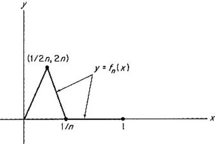
Figure 4.18
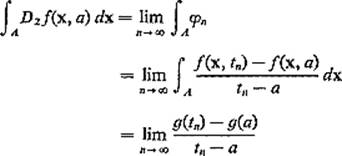
(3)Differentiating under the integral. Let f : A × J → ![]() be a continuous function, where
be a continuous function, where ![]() is contented and
is contented and ![]() is an open interval. Define the partial derivative D2f : A × J →
is an open interval. Define the partial derivative D2f : A × J → ![]() by
by
![]()
and the function g : J → ![]() by g(t) = ∫Af(x, t) dx. We ask whether
by g(t) = ∫Af(x, t) dx. We ask whether
![]()
that is, whether
![]()
According to Exercise 3.5, this is true if D2f is uniformly continuous on A × J. Since differentiation is also a limit operation, this is another “interchange of limit operations” result.
Exercises
3.1(a) If f is integrable, prove that f2 is integrable. Hint: Given ε > 0, let h and k be step functions such that ![]() and ∫(k − h) < ε/M, where M is the maximum value of
and ∫(k − h) < ε/M, where M is the maximum value of ![]() k(x) + h(x)
k(x) + h(x)![]() . Then prove that h2 and k2 are step functions with
. Then prove that h2 and k2 are step functions with ![]() (we may assume that
(we may assume that ![]() since f is integrable if and only if
since f is integrable if and only if ![]() f
f![]() is—why?), and that ∫ (k2 − h2) < ε. Then apply Theorem 3.3.
is—why?), and that ∫ (k2 − h2) < ε. Then apply Theorem 3.3.
(b) If f and g are integrable, prove that fg is integrable. Hint: Express fg in terms of (f + g)2 and (f − g)2; then apply (a).
3.2Let f : ![]() n →
n → ![]() be a bounded function which vanishes outside the interval Q. Show that f is integrable with ∫ f = I if and only if
be a bounded function which vanishes outside the interval Q. Show that f is integrable with ∫ f = I if and only if
![]()
for every sequence of partitions ![]() and associated selections
and associated selections ![]() such that limk→∞ (mesh of
such that limk→∞ (mesh of ![]() k) = 0.
k) = 0.
3.3Let A and B be contented sets, and f : A × B → ![]() a uniformly continuous function. If g : A →
a uniformly continuous function. If g : A → ![]() is defined by
is defined by
![]()
prove that g is continuous. Hint: Write g(x) − g(a) = ∫B [f(x, y) − f(a, y)] dy and apply the uniform continuity of f.
3.4Let ![]() be a sequence of integrable functions which converges uniformly on the contented set A to the integrable function f. Then prove that
be a sequence of integrable functions which converges uniformly on the contented set A to the integrable function f. Then prove that
![]()
Hint: Note that ![]() .
.
3.5Let f : A × J → ![]() be a continuous function, where
be a continuous function, where ![]() is contented and
is contented and ![]() is an open interval. Suppose that
is an open interval. Suppose that ![]() is uniformly continuous on A × J. If
is uniformly continuous on A × J. If
![]()
prove that
![]()
Outline: It suffices to prove that, if ![]() is a sequence of distinct points of J converging to a
is a sequence of distinct points of J converging to a ![]() J, then
J, then
![]()
For each fixed J converging to x ![]() A, the mean value theorem gives
A, the mean value theorem gives ![]() such that
such that
![]()
Let
![]()
Now the hypothesis that D2f is uniformly continuous implies that the sequence ![]() converges uniformly on A to the function D2 f(x, a) of x (explain why). Therefore, by the previous problem, we have
converges uniformly on A to the function D2 f(x, a) of x (explain why). Therefore, by the previous problem, we have
as desired.
3.6Let f : [a, b] × [c, d] → ![]() be a continuous function. Prove that
be a continuous function. Prove that
![]()
by computing the derivatives of the two functions g, h : [a, b] → ![]() defined by
defined by
![]()
and
![]()
using Exercise 3.5 and the fundamental theorem of calculus. This is still another interchange of limit operations.
3.7For each positive integer n, the Bessel function Jn(x) may be defined by
![]()
Prove that Jn(x) satisfies Bessel's differential equation
![]()
3.8Establish the conclusion of Exercise 3.4 without the hypothesis that the limit function f is integrable. Hint: Let Q be a rectangle containing A, and use Theorem 3.4 as follows to prove that f must be integrable. Note first that I = lim ∫ fn exists because ![]() is a Cauchy sequence of real numbers (why?).
is a Cauchy sequence of real numbers (why?).
Given ε > 0, choose N such that both ![]() I − ∫ fN
I − ∫ fN![]() < ε/3 and
< ε/3 and ![]() f(x) − fN(x)
f(x) − fN(x)![]() < ε/3v(Q) for all x. Then choose δ > 0 such that, for any partition
< ε/3v(Q) for all x. Then choose δ > 0 such that, for any partition ![]() of mesh < δ and any selection
of mesh < δ and any selection ![]() ,
,
![]()
Noting that
![]()
also, conclude that
![]()
as desired.
The following example shows that the uniform convergence of ![]() is necessary. Let
is necessary. Let ![]() be the set of all rational numbers in the unit interval [0, 1]. If fn denotes the characteristic function of the set {r1, . . . , rn}, then
be the set of all rational numbers in the unit interval [0, 1]. If fn denotes the characteristic function of the set {r1, . . . , rn}, then ![]() for each n = 1, 2, . . . , but the limit function
for each n = 1, 2, . . . , but the limit function
![]()
is not integrable. The point is that the convergence of this sequence ![]() is not uniform.
is not uniform.
3.9If ![]() , apply Exercise 3.5, the fundamental theorem of calculus, and the chain rule to prove Leibniz' rule:
, apply Exercise 3.5, the fundamental theorem of calculus, and the chain rule to prove Leibniz' rule:
![]()
under appropriate hypotheses (state them).