Advanced Calculus of Several Variables (1973)
Part IV. Multiple Integrals
Chapter 4. ITERATED INTEGRALS AND FUBINI'S THEOREM
If f is a continuous function on the rectangle ![]() , then
, then
![]()
by Exercise 3.6. According to the main theorem of this section, the integral ∫Rf is equal to the common value in (1). Thus ∫Rf may be computed as the result of two “iterated” single-variable integrations (which are easy, using the fundamental theorem of calculus, provided that the necessary antiderivatives can be found). In a similar way, the integral over an interval in ![]() n of a continuous function of n variables can be computed as the result of n iterated single-variable integrations (as we shall see).
n of a continuous function of n variables can be computed as the result of n iterated single-variable integrations (as we shall see).
In introductory calculus, the fact, that
![]()
is usually presented as an application of a “volume by cross-sections” approach. Given ![]() , let
, let
![]()
so At is the “cross-section” in which the plane y = t intersects the ordinate set of f : R → ![]() (see Fig. 4.19). One envisions the ordinate set of f as being swept
(see Fig. 4.19). One envisions the ordinate set of f as being swept
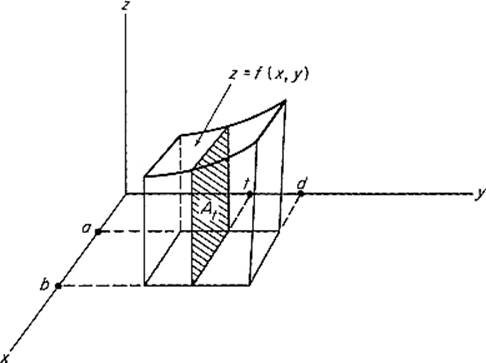
Figure 4.19
out by At as t increases from c to d. Let A(t) denote the area of At, and V(t) the volume over [a, b] × [c, t] = Rt, that is,
![]()
If one accepts the assertion that
![]()
then (2) follows easily. Since
![]()
(3) and the fundamental theorem of calculus give
![]()
So
![]()
because V(c) = 0 gives C = 0. Then
![]()
as desired.
It is the fact, that V′(t) = A(t), for which a heuristic argument is sometimes given at the introductory level. To prove this, assuming that f is continuous on R, let
![]()
Then φ and ψ are continuous functions of (x, h) and
![]()
We temporarily fix t and h, and regard φ and ψ as functions of x, for x ![]() [a, b]. It is clear from the definitions of φ and ψ that the volume between At and At+h under z = f(x, y) contains the set
[a, b]. It is clear from the definitions of φ and ψ that the volume between At and At+h under z = f(x, y) contains the set
![]()
and is contained in the set
![]()
The latter two sets are both “cylinders” of height h, with volumes
![]()
respectively. Therefore
![]()
We now divide through by h and take limits as h → 0. Since Exercise 3.3 permits us to take the limit under the integral signs, substitution of (4) gives
![]()
so V′(t) = A(t) as desired. This completes the proof of (2) if f is continuous on R.
However the hypothesis that f is continuous on R is too restrictive for most applications. For example, in order to reduce ∫Af to iterated integrals, we would choose an interval R containing the contented set A, and define
![]()
Then ∫Af = ∫R g. But even if f is continuous on A, g will in general fail to be continuous at points of ∂A (see Fig. 4.20).
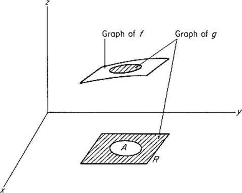
Figure 4.20
The following version of what is known as “Fubini's Theorem” is sufficiently general for our purposes. Notice that the integrals in its statement exist by the remark that, if g : ![]() k →
k → ![]() is integrable and
is integrable and ![]() is contented, then ∫C g exists, because the product of the integrable functions g and φC is integrable by Exercise 3.1.
is contented, then ∫C g exists, because the product of the integrable functions g and φC is integrable by Exercise 3.1.
Theorem 4.1 Let f : ![]() m+n =
m+n = ![]() m ×
m × ![]() n →
n → ![]() be an integrable function such that, for each
be an integrable function such that, for each ![]() , the function fx :
, the function fx : ![]() n →
n → ![]() , defined by fx(y) = f(x, y), is integrable. Given contented sets
, defined by fx(y) = f(x, y), is integrable. Given contented sets ![]() and
and ![]() , let F :
, let F : ![]() m→
m→ ![]() be defined by
be defined by
![]()
Then F is integrable, and
![]()
That is, in the usual notation,
![]()
REMARK The roles of x and y in this theorem can, of course, be interchanged. That is,
![]()
under the hypothesis that, for each ![]() , the function fy :
, the function fy : ![]() n →
n → ![]() , defined by fy(x) = f(x, y), is integrable.
, defined by fy(x) = f(x, y), is integrable.
PROOFWe remark first that it suffices to prove the theorem under the assumption that f(x, y) = 0 unless ![]() . For if f* = fφA × B, fx* = fx φB, and F* = ∫ fx*, then
. For if f* = fφA × B, fx* = fx φB, and F* = ∫ fx*, then
![]()
In essence, therefore, we may replace A, B, and A × B by ![]() m,
m, ![]() n, and
n, and ![]() m × n throughout the proof.
m × n throughout the proof.
We shall employ step functions via Theorem 3.3. First note that, if φ is the characteristic function of an interval ![]() , then
, then
From this it follows that, if ![]() is a step function, then
is a step function, then
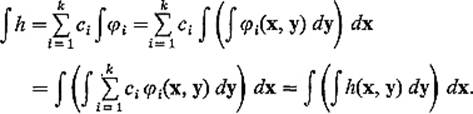
So the theorem holds for step functions.
Now, given ε > 0, let h and k be step functions such that ![]() and ∫ (h − k) < ε. Then for each x we have
and ∫ (h − k) < ε. Then for each x we have ![]() . Hence, if
. Hence, if
![]()
then H and K are step functions on ![]() m such that
m such that ![]() and
and
![]()
by the fact that we have proved the theorem for step functions. Since ε > 0 is arbitrary, Theorem 3.3 now implies that F is integrable, with ![]() . Since we now have ∫f and ∫ F both between ∫ h = ∫ H and ∫ k = ∫ K, and the latter integrals differ by < ε, it follows that
. Since we now have ∫f and ∫ F both between ∫ h = ∫ H and ∫ k = ∫ K, and the latter integrals differ by < ε, it follows that
![]()
This being true for all ε > 0, the proof is complete.
![]()
The following two applications of Fubini's theorem are generalizations of methods often used in elementary calculus courses either to define or to calculate volumes. The first one generalizes to higher dimensions the method of “volumes by cross-sections.”
Theorem 4.2 (Cavalieri's Principle) Let A be a contented subset of ![]() n+1, with
n+1, with ![]() , where
, where ![]() and
and ![]() are intervals. Suppose
are intervals. Suppose
![]()
is contented for each t ![]() [a, b], and write A(t) = v(At). Then
[a, b], and write A(t) = v(At). Then
![]()
PROOF(see Fig. 4.21).
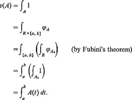
![]()
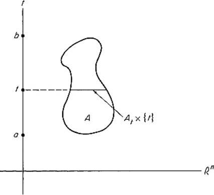
Figure 4.21
The most typical application of Cavalieri's principle is to the computation of volumes of revolution in ![]() 3. Let f : [a, b] →
3. Let f : [a, b] → ![]() be a positive continuous function. Denote by A the set in
be a positive continuous function. Denote by A the set in ![]() 3 obtained by revolving about the x-axis the ordinate set of f (Fig. 4.22). It is clear that A(t) = π[f(t)]2, so Theorem 4.2 gives
3 obtained by revolving about the x-axis the ordinate set of f (Fig. 4.22). It is clear that A(t) = π[f(t)]2, so Theorem 4.2 gives
![]()
For example, to compute the volume of the 3-dimensional ball Br3 of radius r, take f(x) = (r2 − x2)1/2 on [−r, r]. Then we obtain
![]()
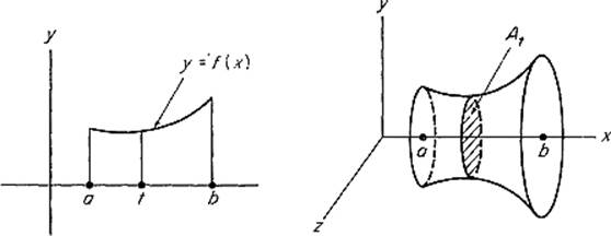
Figure 4.22
Theorem 4.3If ![]() is a contented set, and f1 and f2 are continuous functions on A such that
is a contented set, and f1 and f2 are continuous functions on A such that ![]() , then
, then
![]()
is a contented set. If g : C → ![]() is continuous, then
is continuous, then
![]()
PROOF The fact that C is contented follows easily from Corollary 2.3. Let B be a closed interval in ![]() containing
containing ![]() , so that
, so that ![]() (see Fig. 4.23).
(see Fig. 4.23).

Figure 4.23
If h gφc, then it is clear that the functions h : ![]() n+1 →
n+1 → ![]() and hx :
and hx : ![]() →
→ ![]() are admissible, so Fubini's theorem gives
are admissible, so Fubini's theorem gives
![]()
because hx(y) = 1 if ![]() , and 0 otherwise.
, and 0 otherwise.
![]()
For example, if g is a continuous function on the unit ball ![]() , then
, then
![]()
where ![]() .
.
The case m = n = 1 of Fubini's theorem, with A = [a, b] and B = [c, d], yields the formula
![]()
alluded to at the beginning of this section. Similarly, if f : Q → ![]() is continuous, and Q = [a1, b1] × · · · × [an, bn] is an interval in
is continuous, and Q = [a1, b1] × · · · × [an, bn] is an interval in ![]() n, then n − 1 applications of Fubini's theorem yield the formula
n, then n − 1 applications of Fubini's theorem yield the formula
![]()
This is the computational significance of Fubini's theorem—it reduces a multivariable integration over an interval in ![]() n to a sequence of n successive single-variable integrations, in each of which the fundamental theorem of calculus can be employed.
n to a sequence of n successive single-variable integrations, in each of which the fundamental theorem of calculus can be employed.
If Q is not an interval, it may be possible, by appropriate substitutions, to “transform” ∫Q f to an integral ∫R g, where R is an interval (and then evaluate ∫R g by use of Fubini's theorem and the fundamental theorem of calculus). This is the role of the “change of variables formula” of the next section.
Exercises
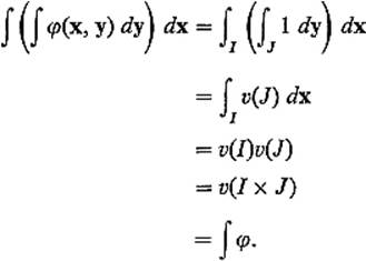
4.1Let ![]() and
and ![]() be contented sets, and f :
be contented sets, and f : ![]() m →
m → ![]() and g :
and g : ![]() n →
n → ![]() integrable functions. Define h :
integrable functions. Define h : ![]() m + n →
m + n → ![]() by h(x, y) = f(x)g(y), and prove that
by h(x, y) = f(x)g(y), and prove that
![]()
Conclude as a corollary that v(A × B) = v(A)v(B).
4.2Use Fubini‘s theorem to give an easy proof that ∂2f/∂x ∂y = ∂2f/∂y ∂x if these second derivatives are both continuous. Hint: If D1 D2f − D2 D1f > 0 at some point, then there is a rectangle R on which it is positive. However use Fubini’s theorem to calculate ∫R (D1 D2f − D2 D1f) = 0.
4.3Define f : I × I → ![]() , I = {0, 1} by
, I = {0, 1} by
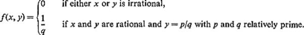
Then show that
(a) ![]()
(b) ![]()
(c) ![]() if y is irrational, but does not exist if y is rational.
if y is irrational, but does not exist if y is rational.
4.4Let T be the solid torus in ![]() 3 obtained by revolving the circle
3 obtained by revolving the circle ![]() , in the yz-plane, about the z-axis. Use Cavalieri's principle to compute v(T) = 2π2ab2.
, in the yz-plane, about the z-axis. Use Cavalieri's principle to compute v(T) = 2π2ab2.
4.5Let S be the intersection of the cylinders ![]() and
and ![]() . Use Cavalieri's principle to compute
. Use Cavalieri's principle to compute ![]() .
.
4.6The area of the ellipse ![]() , with semiaxes a and b, is A = πab. Use this fact and Cavalieri's principle to show that the volume enclosed by the ellipsoid
, with semiaxes a and b, is A = πab. Use this fact and Cavalieri's principle to show that the volume enclosed by the ellipsoid
![]()
is ![]() . Hint: What is the area A(t) of the ellipse of intersection of the plane x = t and the ellipsoid? What are the semiaxes of this ellipse?
. Hint: What is the area A(t) of the ellipse of intersection of the plane x = t and the ellipsoid? What are the semiaxes of this ellipse?
4.7Use the formula ![]() , for the volume of a 3-dimensional ball of radius r, and Cavalieri's principle, to show that the volume of the 4-dimensional unit ball
, for the volume of a 3-dimensional ball of radius r, and Cavalieri's principle, to show that the volume of the 4-dimensional unit ball ![]() is π2/2. Hint: What is the volume A(t) of the 3-dimensional ball in which the hyperplane x4 = t intersects B4?
is π2/2. Hint: What is the volume A(t) of the 3-dimensional ball in which the hyperplane x4 = t intersects B4?
4.8Let C be the 4-dimensional “solid cone” in ![]() 4 that is bounded above by the 3-dimensional ball of radius a that is centered at (0, 0, 0, h) in the hyperplane x4 = h, and below by the conical “surface” x4 = (x12 + x22 + x22)1/2. Show that
4 that is bounded above by the 3-dimensional ball of radius a that is centered at (0, 0, 0, h) in the hyperplane x4 = h, and below by the conical “surface” x4 = (x12 + x22 + x22)1/2. Show that ![]() . Note that this is one-fourth times the height of the cone C times the volume of its base.
. Note that this is one-fourth times the height of the cone C times the volume of its base.