Advanced Calculus of Several Variables (1973)
Part IV. Multiple Integrals
Chapter 5. CHANGE OF VARIABLES
The student has undoubtedly seen change of variables formulas such as
![]()
and
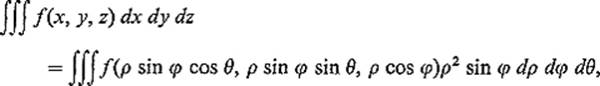
which result from changes from rectangular coordinates to polar and spherical coordinates respectively. The appearance of the factor r in the first formula and the factor ρ2 sin φ in the second one is sometimes “explained” by mythical pictures, such as Figure 4.24, in which it is alleged that dA is an “infinitesimal”
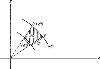
Figure 4.24
rectangle with sides dr and r dθ, and therefore has area r dr dθ. In this section we shall give a mathemtaically acceptable explanation of the origin of such factors in the transformation of multiple integrals from one coordinate system to another.
This will entail a thorough discussion of the technique of substitution for multivariable integrals. The basic problem is as follows. Let T : ![]() n →
n → ![]() n be a mapping which is
n be a mapping which is ![]() (continuously differentiable) and also
(continuously differentiable) and also ![]() -invertible on some neighborhood U of the set
-invertible on some neighborhood U of the set ![]() , meaning that T is one-to-one on U and that T−1 : T(U) → U is also a
, meaning that T is one-to-one on U and that T−1 : T(U) → U is also a ![]() mapping. Given an integrable function f : T(A) →
mapping. Given an integrable function f : T(A) → ![]() , we would like to “transform” the integral ∫T(A) f into an appropriate integral over A (which may be easier to compute).
, we would like to “transform” the integral ∫T(A) f into an appropriate integral over A (which may be easier to compute).
For example, suppose we wish to compute ∫Q f, where Q is an annular sector in the plane ![]() 2, as pictured in Fig. 4.25. Let T :
2, as pictured in Fig. 4.25. Let T : ![]() 2 →
2 → ![]() 2 be the “polar coordinates” mapping defined by T(r, θ) = (r cos θ, r sin θ). Then Q = T(A), where A is the rectangle
2 be the “polar coordinates” mapping defined by T(r, θ) = (r cos θ, r sin θ). Then Q = T(A), where A is the rectangle ![]() . If ∫Q f can be transformed into an integral over A then, because A is a rectangle, the latter integral will be amenable to computation by iterated integrals (Fubini's theorem).
. If ∫Q f can be transformed into an integral over A then, because A is a rectangle, the latter integral will be amenable to computation by iterated integrals (Fubini's theorem).
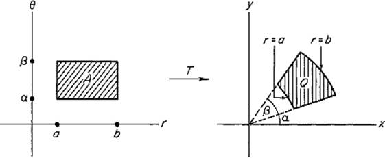
Figure 4.25
The principal idea in this discussion will be the local approximation of the transformation T by its differential linear mapping dT. Recall that dTa : ![]() n →
n → ![]() n is that linear mapping which “best approximates” the mapping h → T(a + h) − T(a) in a neighborhood of the point
n is that linear mapping which “best approximates” the mapping h → T(a + h) − T(a) in a neighborhood of the point ![]() , and that the matrix of dTa is the derivative matrix T′(a) = (DjTi(a)), where T1, . . . , Tn are the component functions of T :
, and that the matrix of dTa is the derivative matrix T′(a) = (DjTi(a)), where T1, . . . , Tn are the component functions of T : ![]() n →
n → ![]() n.
n.
We therefore discuss first the behavior of volumes under linear distortions. That is, given a linear mapping λ : ![]() n →
n → ![]() n and a contented set
n and a contented set ![]() , we investigate the relationship between v(A) and v(λ(A)) [assuming, as we will prove, that the image λ(A) is also contented]. If λ is represented by the n × n matrix A, that is, λ(x) = Ax, we write
, we investigate the relationship between v(A) and v(λ(A)) [assuming, as we will prove, that the image λ(A) is also contented]. If λ is represented by the n × n matrix A, that is, λ(x) = Ax, we write
![]()
Theorem 5.1 If λ : ![]() n →
n → ![]() n is a linear mapping, and
n is a linear mapping, and ![]() is contented, then λ(B) is also contented, and
is contented, then λ(B) is also contented, and
![]()
PROOFFirst suppose that det λ = 0, so the column vectors of the matrix of λ are linearly dependent (see by Theorem I.6.1). Since these column vectors are the images under λ of the standard unit vectors e1, . . . , en in ![]() n, it then follows that λ(
n, it then follows that λ(![]() n) is a proper subspace of
n) is a proper subspace of ![]() n. Since it is easily verified that any bounded subset of a proper subspace of
n. Since it is easily verified that any bounded subset of a proper subspace of ![]() n is negligible (Exercise 5.1), we see that (1) is trivially satisfied if det λ = 0.
n is negligible (Exercise 5.1), we see that (1) is trivially satisfied if det λ = 0.
If det λ ≠ 0, then a standard theorem of linear algebra asserts that the matrix A of λ can be written as a product
![]()
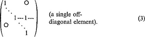
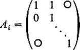
where each Ai is either of the form
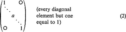
or of the form
Hence λ is a composition λ = λ1 ![]() λ2
λ2 ![]() · · ·
· · · ![]() λk, where λi is the linear mapping represented by the matrix Ai.
λk, where λi is the linear mapping represented by the matrix Ai.
If Ai is of the form (2), with a appearing in the pth row and column, then
![]()
so it is clear that, if I is an interval, then λi(I) is also an interval, with v(λi(I)) = ![]() a
a![]() v(I). From this, and the definition of volume in terms of intervals, it follows easily that, if B is a contented set, then λi(B) is contented with v(λi(B)) =
v(I). From this, and the definition of volume in terms of intervals, it follows easily that, if B is a contented set, then λi(B) is contented with v(λi(B)) = ![]() a
a![]() v(B) =
v(B) = ![]() det λi
det λi![]() v(B).
v(B).
We shall show below that, if Ai is of the form (3), then v(λi(B)) = v(B) = ![]() det λi
det λi![]() v(B) for any contented set. Granting this, the theorem follows, because we then have
v(B) for any contented set. Granting this, the theorem follows, because we then have
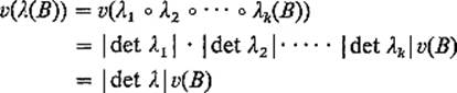
as desired, since the determinant of a product of matrices is the product of their determinants.
So it remains only to verify that λi preserves volumes if the matrix Ai of λi is of the form (3). We consider the typical case in which the off-diagonal element of Ai is in the first row and second column, that is,
so
![]()
We show first that λi preserves the volume of an interval
![]()
If we write I = I′ × I″ where ![]() and
and ![]() , then (4) shows that
, then (4) shows that
![]()
where I* is the pictured parallelogram in ![]() 2 (Fig. 4.26). Since it is clear that v(I*) = v(I′), Exercise 4.1 gives
2 (Fig. 4.26). Since it is clear that v(I*) = v(I′), Exercise 4.1 gives
![]()
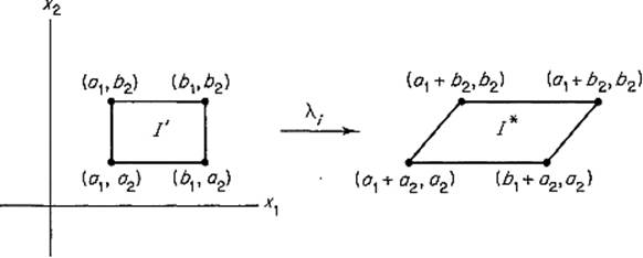
Figure 4.26
Now let B be a contented set in ![]() n, and, given ε > 0, consider nonoverlapping intervals I1, . . . , Ip and intervals J1, . . . , Jq such that
n, and, given ε > 0, consider nonoverlapping intervals I1, . . . , Ip and intervals J1, . . . , Jq such that
![]()
and
![]()
Since we have seen that λi preserves the volumes of intervals, we then have
![]()
and
![]()
Finally it follows easily from these inequalities that λi(B) is contented, with v(λi(B)) = v(B) as desired (see Exercise 5.2).
![]()
We are now in a position to establish the invariance of volume under rigid motions.
Corollary 5.2 If ![]() is a contented set and ρ :
is a contented set and ρ : ![]() n →
n → ![]() n is a rigid motion, then ρ(A) is contented and v(ρ(A)) = v(A).
n is a rigid motion, then ρ(A) is contented and v(ρ(A)) = v(A).
The statement that ρ is a rigid motion means that ρ = τa ![]() μ, where τa is the translation by a, τa(x) = x + a, and μ is an orthogonal transformation, so that
μ, where τa is the translation by a, τa(x) = x + a, and μ is an orthogonal transformation, so that ![]() det μ
det μ ![]() = 1 (see Exercise 1.6.10). The fact that ρ(A) is contented with v(ρ(A)) = v(A) therefore follows immediately from Theorem 5.1.
= 1 (see Exercise 1.6.10). The fact that ρ(A) is contented with v(ρ(A)) = v(A) therefore follows immediately from Theorem 5.1.
Example 1 Consider the ball
![]()
of radius r in ![]() n. Note that Brn is the image of the unit n-dimensional ball
n. Note that Brn is the image of the unit n-dimensional ball ![]() under the linear mapping T(x) = rx. Since
under the linear mapping T(x) = rx. Since ![]() det T′
det T′ ![]() =
= ![]() det T
det T ![]() = rn, Theorem 5.1 gives
= rn, Theorem 5.1 gives
![]()
Thus the volume of an n-dimensional ball is proportional to the nth power of its radius. Let αn denote the volume of the unit n-dimensional ball B1n, so
![]()
In Exercises 5.17, 5.18, and 5.19, we shall see that
![]()
These formulas are established by induction on m, starting with the familiar α2 = π and α3 = 4π/3.
In addition to the effect on volumes of linear distortions, discussed above, a key ingredient in the derivation of the change of variables formula is the fact that, if F : ![]() n →
n → ![]() n is a
n is a ![]() mapping such that dF0 = I (the identity transformation of
mapping such that dF0 = I (the identity transformation of ![]() n), then in a sufficiently small neighborhood of 0, F differs very little from the identity mapping, and in particular does not significantly alter the volumes of sets within this neighborhood.
n), then in a sufficiently small neighborhood of 0, F differs very little from the identity mapping, and in particular does not significantly alter the volumes of sets within this neighborhood.
This is the effect of the following lemma, which was used in the proof of the inverse function theorem in Chapter III. Recall that the norm ![]() λ
λ![]() of the linear mapping λ :
of the linear mapping λ : ![]() n →
n → ![]() n is by definition the maximum value of
n is by definition the maximum value of ![]() λ(x)
λ(x)![]() 0 for all
0 for all ![]() , where
, where
![]()
and ![]() . Thus Cr is a “cube” centered at 0 with (r, r, . . . , r) as one vertex, and is referred to as “the cube of radius r centered at the origin.”
. Thus Cr is a “cube” centered at 0 with (r, r, . . . , r) as one vertex, and is referred to as “the cube of radius r centered at the origin.”
The lemma then asserts that, if dFx differs (in norm) only slightly from the identity mapping I for all ![]() , then the image F(Cr) contains a cube slightly smaller than Cr, and is contained in one slightly larger than Cr.
, then the image F(Cr) contains a cube slightly smaller than Cr, and is contained in one slightly larger than Cr.
Lemma 5.3 (Lemma III.3.2) Let U be an open set in ![]() n containing Cr, and F : U →
n containing Cr, and F : U → ![]() n a
n a ![]() mapping such that F(0) = 0 and dF0 = I. Suppose also that there exists
mapping such that F(0) = 0 and dF0 = I. Suppose also that there exists ![]() such that
such that
![]()
for all ![]() . Then
. Then
![]()
(see Fig. 4.27).
Now let Q be an interval centered at the point ![]() , and suppose that T : U →
, and suppose that T : U → ![]() n is a
n is a ![]() -invertible mapping on a neighborhood U of Q. Suppose in addition that the differential dTx is almost constant on Q, dTx ≈ dTa, and in particular that
-invertible mapping on a neighborhood U of Q. Suppose in addition that the differential dTx is almost constant on Q, dTx ≈ dTa, and in particular that
![]()
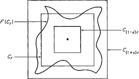
Figure 4.27
for all x ![]() Q. Also let Q1−ε and Q1+ε be intervals centered at a and both “similar” to Q, with each edge of Q1±ε equal (in length) to 1 ± ε times the corresponding edge of Q, so v(Q1±ε) = (1 ± ε)nv(Q). (see Fig. 4.28.)
Q. Also let Q1−ε and Q1+ε be intervals centered at a and both “similar” to Q, with each edge of Q1±ε equal (in length) to 1 ± ε times the corresponding edge of Q, so v(Q1±ε) = (1 ± ε)nv(Q). (see Fig. 4.28.)
Then the idea of the proof of Theorem 5.4 below is to use Lemma 5.3 to show that (6) implies that the image set T(Q) closely approximates the “parallelepiped” dTa(Q), in the sense that
![]()
It will then follow from Theorem 5.1 that
![]()
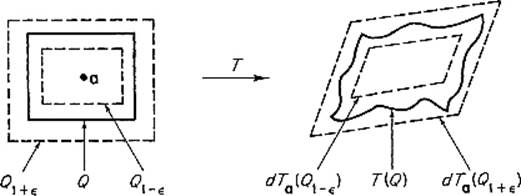
Figure 4.28
Theorem 5.4 Let Q be an interval centered at the point ![]() , and suppose T : U →
, and suppose T : U → ![]() n is a
n is a ![]() -invertible mapping on a neighborhood U of Q. If there exists
-invertible mapping on a neighborhood U of Q. If there exists ![]() such that
such that
![]()
for all x ![]() Q, then T(Q) is contented with
Q, then T(Q) is contented with
![]()
PROOFWe leave to Exercise 5.3 the proof that T(Q) is contented, and proceed to verify (7).
First suppose that Q is a cube of radius r. Let τa denote translation by a, τa(x) = a + x, so τa(Cr) = Q. Let b = T(a), and λ = dTa. Let F = λ−1 ![]() τb−1
τb−1 ![]() T
T ![]() τa (see Fig. 4.29).
τa (see Fig. 4.29).
By the chain rule we obtain
![]()
Since the differential of a translation is the identity mapping, this gives
![]()
for all ![]() . Consequently hypothesis (6) implies that F : Cr →
. Consequently hypothesis (6) implies that F : Cr → ![]() n satisfies (5). Consequently Lemma 5.3 applies to yield
n satisfies (5). Consequently Lemma 5.3 applies to yield
![]()
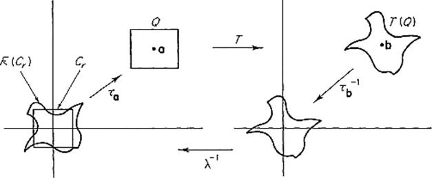
Figure 4.29
so
![]()
Since ![]() , Theorem 5.1 implies that
, Theorem 5.1 implies that
![]()
Since v(Q) = v(Cr), we therefore obtain (7) upon multiplication of (8) by ![]() det T′(a)
det T′(a)![]() . This completes the proof in case Q is a cube.
. This completes the proof in case Q is a cube.
If Q is not a cube, let ρ : ![]() n →
n → ![]() n be a linear mapping such that ρ(C1) is congruent to Q, and τa
n be a linear mapping such that ρ(C1) is congruent to Q, and τa ![]() ρ(C1) = Q in particular. Then v(Q) =
ρ(C1) = Q in particular. Then v(Q) = ![]() det ρ
det ρ ![]() v(C1) by Theorem 5.1. Let
v(C1) by Theorem 5.1. Let
![]()
Then the chain rule gives
![]()
because dρ = ρ since ρ is linear. Therefore
![]()
by (6), so S : C1 → ![]() n itself satisfies the hypothesis of the theorem, with C1 a cube.
n itself satisfies the hypothesis of the theorem, with C1 a cube.
What we have already proved therefore gives
![]()
Since S(C1) = T(Q) and
![]()
this last inequality is (7) as desired.
![]()
Since (1 ± ε)n ≈ 1 if ε is very small, the intuitive content of Theorem 5.4 is that, if dTx is approximately equal to dTa for all x ![]() Q (and this should be true if Q is sufficiently small), then v(T(Q)) is approximately equal to
Q (and this should be true if Q is sufficiently small), then v(T(Q)) is approximately equal to ![]() det T′(a)
det T′(a)![]() v(Q). Thus the factor
v(Q). Thus the factor ![]() det T′(a)
det T′(a)![]() seems to play the role of a “local magnification factor.” With this interpretation of Theorem 5.4, we can now give a heuristic derivation of the change of variables formula for multiple integrals.
seems to play the role of a “local magnification factor.” With this interpretation of Theorem 5.4, we can now give a heuristic derivation of the change of variables formula for multiple integrals.
Suppose that T : ![]() n →
n → ![]() n is
n is ![]() -invertible on a neighborhood of the interval Q, and suppose that f :
-invertible on a neighborhood of the interval Q, and suppose that f : ![]() n →
n → ![]() is an integrable function such that f
is an integrable function such that f ![]() T is also integrable.
T is also integrable.
Let ![]() = {Q1, . . . , Qk} be a partition of Q into very small subintervals, and
= {Q1, . . . , Qk} be a partition of Q into very small subintervals, and ![]() = {a1, . . . , ak} the selection for
= {a1, . . . , ak} the selection for ![]() such that ai is the center-point of Qi (Fig. 4.30). Then
such that ai is the center-point of Qi (Fig. 4.30). Then
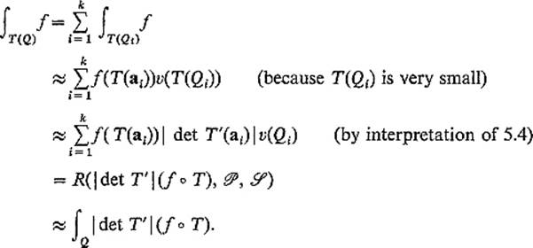
The proof of the main theorem is a matter of supplying enough epsilonics to convert the above discussion into a precise argument.
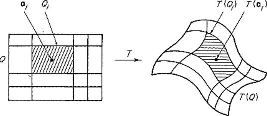
Figure 4.30
Theorem 5.5Let Q be an interval in ![]() n, and T :
n, and T : ![]() n →
n → ![]() n a mapping which is
n a mapping which is ![]() -invertible on a neighborhood of Q. If f :
-invertible on a neighborhood of Q. If f : ![]() n →
n → ![]() is an integrable function such that f
is an integrable function such that f ![]() T is also integrable, then
T is also integrable, then
![]()
PROOFLet η > 0 be given to start with. Given a partition ![]() = {Q1, . . . , Qk} of Q, let
= {Q1, . . . , Qk} of Q, let ![]() = {a1, . . . , ak} be the selection consisting of the center-points of the intervals of
= {a1, . . . , ak} be the selection consisting of the center-points of the intervals of ![]() . By Theorem 3.4 there exists δ1 > 0 such that
. By Theorem 3.4 there exists δ1 > 0 such that
![]()
if mesh ![]() < δ1, where R denotes the Riemann sum
< δ1, where R denotes the Riemann sum
![]()
Choose A > 0 and M > 0 such that
![]()
for all x ![]() Q. This is possible because det T′(x) is continuous (hence bounded) on Q, and f
Q. This is possible because det T′(x) is continuous (hence bounded) on Q, and f ![]() T is integrable (hence bounded) on Q. If
T is integrable (hence bounded) on Q. If
![]()
then
![]()
where
![]()
By Theorem 3.4 there exists δ2 > 0 such that, if mesh ![]() < δ2, then any two Riemann sums for f
< δ2, then any two Riemann sums for f ![]() T on
T on ![]() differ by less than η/6A, because each differs from ∫Qf
differ by less than η/6A, because each differs from ∫Qf ![]() T by less than η/12A. It follows that
T by less than η/12A. It follows that
![]()
because there are Riemann sums for f ![]() T arbitrarily close to both
T arbitrarily close to both ![]() and
and ![]() . Hence (11) and (12) give
. Hence (11) and (12) give
![]()
because each Δi < A. Summarizing our progress thus far, we have the Riemann sum R which differs from ∫Q (f ![]() T)
T)![]() det T′
det T′![]() by less than η/2, and lies between the two numbers α and β, which in turn differ by less than η/6.
by less than η/2, and lies between the two numbers α and β, which in turn differ by less than η/6.
Next we want to locate ∫T(Q)f between two numbers α′ and β′ which are close to α and β, respectively. Since the sets T(Qi) are contented (by Exercise 5.3) and intersect only in their boundaries,
![]()
by Proposition 2.7. Therefore
![]()
by Proposition 2.5. Our next task is to estimate α′ − α and β′ − β, and this is where Theorem 5.4 will come into play.
Choose ![]() such that
such that
![]()
Since T is ![]() -invertible in a neighborhood of Q, we can choose an upper bound B for the value of the norm
-invertible in a neighborhood of Q, we can choose an upper bound B for the value of the norm ![]() . By uniform continuity there exists δ3 > 0 such that, if mesh
. By uniform continuity there exists δ3 > 0 such that, if mesh ![]() < δ3, then
< δ3, then
![]()
for all ![]() . This in turn implies that
. This in turn implies that
for all ![]() . Consequently Theorem 5.4 applies to show that v(T(Qi)) lies between
. Consequently Theorem 5.4 applies to show that v(T(Qi)) lies between
![]()
as does Δi v(Qi).
It follows that
![]()
if the mesh of ![]() is less than δ3. We now fix the partition
is less than δ3. We now fix the partition ![]() with mesh less than δ = min(δ1, δ2, δ3). Then
with mesh less than δ = min(δ1, δ2, δ3). Then
by (15) and (16). Similarly
![]()
We are finally ready to move in for the kill. If α* = min(α, α′) and β* = max(β, β′) then, by (11) and (14), both R and ∫T(Q) f lie between α* and β*.
Since (13), (17), and (18) imply that β* − α* < η/2, it follows that
![]()
Thus ∫T(Q) f and ∫Q (f ![]() T)
T)![]() det T′
det T′![]() both differ from R by less than η/2, so
both differ from R by less than η/2, so
![]()
This being true for every η > 0, we conclude that
![]()
Theorem 5.5 is not quite general enough for some of the standard applications of the change of variables formula. However, the needed generalizations are usually quite easy to come by, the real work having already been done in the proof of Theorem 5.5. For example, the following simple extension will suffice for most purposes.
Addendum 5.6 The conclusion of Theorem 5.5 still holds if the ![]() mapping T :
mapping T : ![]() n →
n → ![]() n is only assumed to be
n is only assumed to be ![]() -invertible on the interior of the interval Q (instead of on a neighborhood of Q).
-invertible on the interior of the interval Q (instead of on a neighborhood of Q).
PROOFLet Q* be an interval interior to Q, and write K = Q − int Q* (Fig. 4.31). Then Theorem 5.5 as stated gives
![]()

Figure 4.31
But
![]()
and
![]()
and the integrals over K and T(K) can be made as small as desired by making the volume of K, and hence that of T(K), sufficiently small. The easy details are left to the student (Exercise 5.4).
![]()
Example 2Let A denote the annular region in the plane bounded by the circles of radii a and b centered at the origin (Fig. 4.32). If T : ![]() 2 →
2 → ![]() 2 is the “polar coordinates mapping” defined by
2 is the “polar coordinates mapping” defined by
![]()
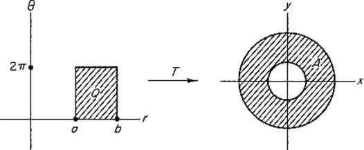
Figure 4.32
(for clarity we use r and θ as coordinates in the domain, and x and y as coordinates in the image), then A is the image under T of the rectangle
![]()
T is not one-to-one on Q, because T(r, 0) = T(r, 2π), but is ![]() -invertible on the interior of Q, so Addendum 5.6 gives
-invertible on the interior of Q, so Addendum 5.6 gives
![]()
Since ![]() det T′(r, θ)
det T′(r, θ)![]() = r, Fubini's theorem then gives
= r, Fubini's theorem then gives
![]()
Example 3Let A be an “ice cream cone” bounded above by the sphere of radius 1 and below by a cone with vertex angle π/6 (Fig. 4.33). If T: ![]() 3 →
3 → ![]() 3 is the “spherical coordinates mapping” defined by
3 is the “spherical coordinates mapping” defined by
![]()
then A is the image under T of the interval
![]()
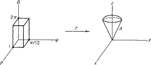
Figure 4.33
T is not one-to-one on Q (for instance, the image under T of the back face ρ = 0 of Q is the origin), but is ![]() -invertible on the interior of Q, so Addendum 5.6 together with Fubini's theorem gives
-invertible on the interior of Q, so Addendum 5.6 together with Fubini's theorem gives
![]()
since ![]() det T′(ρ, φ, θ)
det T′(ρ, φ, θ)![]() = ρ2 sin φ.
= ρ2 sin φ.
Example 4To compute the volume of the unit ball ![]() , take f(x) ≡ 1, T the spherical coordinates mapping of Example 2, and
, take f(x) ≡ 1, T the spherical coordinates mapping of Example 2, and
![]()
Then T(Q) = B3, and T is ![]() -invertible on the interior of Q. Therefore Addendum 5.6 yields
-invertible on the interior of Q. Therefore Addendum 5.6 yields
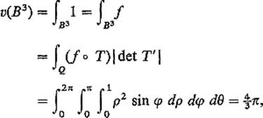
the familiar answer.
In integration problems that display an obvious cylindrical or spherical symmetry, the use of polar or spherical coordinates is clearly indicated. In general, in order to evaluate ∫Rf by use of the change of variables formula, one chooses the transformation T (often in an ad hoc manner) so as to simplify either the function f or the region R (or both). The following two examples illustrate this.
Example 5Suppose we want to compute
![]()
where R is the region in the first quadrant which is bounded by the coordinate axes and the curve ![]() (a parabola). The substitution
(a parabola). The substitution ![]() seems promising (it simplifies the integrand considerably), so we consider the mapping T from uv-space to xy-space defined by x = u2, y = v2 (see Fig. 4.34). It maps onto R the triangle Q in the uv-plane bounded by the co-
seems promising (it simplifies the integrand considerably), so we consider the mapping T from uv-space to xy-space defined by x = u2, y = v2 (see Fig. 4.34). It maps onto R the triangle Q in the uv-plane bounded by the co-
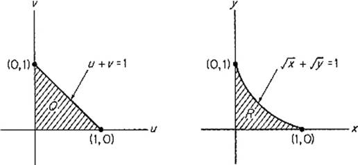
Figure 4.34
ordinate axes and the line u + v = 1. Now det T′ = 4uv, so the change of variables formula (which applies here, by Exercise 5.4) gives
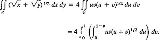
This iterated integral (obtained from Theorem 4.3) is now easily evaluated using integration by substitution (we omit the details).
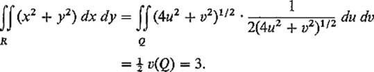
Example 6Consider ∫∫R (x2 + y2) dx dy, where R is the region in the first quadrant that is bounded by the hyperbolas xy = 1, xy = 3, x2 − y2 = 1, and x2 − y2 = 4. We make the substitution u = xy, v = x2 − y2 so as to simplify the region; this transformation S from xy-space to uv-space maps the region R onto the rectangle Q bounded by the lines u = 1, u = 3, v = 1, v = 4 (see Fig. 4.35). From u = xy, v = x2 − y2 we obtain
![]()
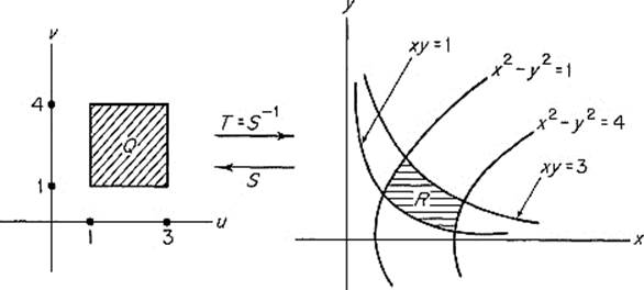
Figure 4.35
The last two equations imply that S is one-to-one on R; we are actually interested in its inverse T = S−1. Since S ![]() T = I, the chain rule gives S′(T(u, v))
T = I, the chain rule gives S′(T(u, v)) ![]() T′(u, v) = I, so
T′(u, v) = I, so
![]()
Consequently the change of variables formula gives
Multiple integrals are often used to compute mass. A body with mass consists of a contented set A and an integrable density function μ : A → ![]() ; its mass M(A) is then defined by
; its mass M(A) is then defined by
![]()
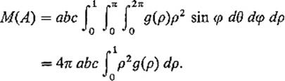
Example 7Let A be the ellipsoidal ball ![]() , with its density function μ being constant on concentric ellipsoids. That is, there exists a function g : [0, 1] →
, with its density function μ being constant on concentric ellipsoids. That is, there exists a function g : [0, 1] → ![]() such that μ(x) = g(ρ) at each point x of the ellipsoid
such that μ(x) = g(ρ) at each point x of the ellipsoid
![]()
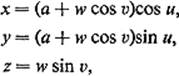
In order to compute M(A), we intoduce ellipsoidal coordinates by
![]()
The transformation T defined by these equations maps onto A the interval
![]()
and is invertible on the interior of Q. Since det T′ = abcρ2 sin φ, Addendum 5.6 gives
For instance, taking g(ρ) ≡ 1 (uniform unit density), we see that the volume of the ellipsoid ![]() is
is ![]() (as seen previously in Exercise 4.6).
(as seen previously in Exercise 4.6).
A related application of multiple integrals is to the computation of force. A force field is a vector-valued function, whereas we have thus far integrated only scalar-valued functions. The function G : ![]() n →
n → ![]() m is said to be integrable on
m is said to be integrable on ![]() if and only if each of its component functions g1, . . . , gm is, in which case we define
if and only if each of its component functions g1, . . . , gm is, in which case we define
![]()
Thus vector-valued functions are simply integrated componentwise.
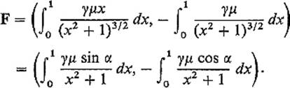
As an example, consider a body A with density function μ : A → ![]() , and let ξ be a point not in A. Motivated by Newton's law of gravitation, we define the gravitational force exerted by A, on a particle of mass m situated at ξ, to be the vector
, and let ξ be a point not in A. Motivated by Newton's law of gravitation, we define the gravitational force exerted by A, on a particle of mass m situated at ξ, to be the vector
![]()
where γ is the “gravitational constant.”
For example, suppose that A is a uniform rod (μ = constant) coincident with the unit interval [0, 1] on the x-axis, and ξ = (0, 1). (see Fig. 4.36.) Then the gravitational force exerted by the rod A on a unit mass at ξ is
For a more interesting example, see Exercises 5.13 and 5.14.
We close this section with a discussion of some of the classical notation and terminology associated with the change of variables formula. Given a differentiable mapping T : ![]() n →
n → ![]() n, recall that the determinant det T′(a) of the deriva-
n, recall that the determinant det T′(a) of the deriva-
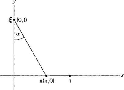
Figure 4.36
tive matrix T′(a) is called the Jacobian (determinant) of T at a. A standard notation (which we have used in Chapter III) for the Jacobian is
![]()
where T1, . . . , Tn are as usual the component functions of T, thought of as a mapping from u-space (with coordinates u1, . . . , un) to x-space (with coordinates x1, . . . , xn). If we replace the component functions T1, . . . , Tn in the Jacobian by the variables x1, . . . , xn which they give,
![]()
then the change of variables formula takes the appealing form
![]()
With the abbreviations
![]()
and
![]()
the above formula takes the simple form
![]()
This form of the change of variables formula is particularly pleasant because it reads the same as the familar substitution rule for single-variable integrals (Theorem 1.7), taking into account the change of sign in a single-variable integral which results from the interchange of its limits of integration.
This observation leads to an interpretation of the change of variables formula as the result of a “mechanical” substitution procedure. Suppose T is a differentiable mapping from uv-space to xy-space. In the integral ∫T(Q) f(x, y) dx dy we want to make the substitutions
![]()
suggested by the chain rule. In formally multiplying together these two “differential forms,” we agree to the conventions
![]()
for no other reason than that they are necessary if we are to get the “right” answer. We then obtain
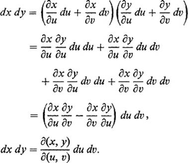
Note that, to within sign, this result agrees with formula (20), according to which dx dy should be replaced by ![]() ∂(x, y)/∂(u, v)
∂(x, y)/∂(u, v)![]() du dv when the integral is transformed.
du dv when the integral is transformed.
Thus the change of variables (x, y) = T(u, v) in a 2-dimensional integral ∫T(Q)f(x, y) dx dy may be carried out in the following way. First replace x and y in f(x, y) by their expressions in terms of u and v, then multiply out dx dy as above using (21) and (22), and finally replace the coefficient of du dv, which is obtained, by its absolute value,
For example, in a change from rectangular to polar coordinates, we have x = r cos θ and y = r sin θ, so
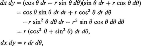
where the sign is correct because ![]() .
.
The relation dv du = −du dv requires a further comment. Once having agreed upon u as the first coordinate and v as the second one, we agree that
![]()
while
![]()
So, in writing multidimensional integrals with differential notation, the order of the differentials in the integrand makes a difference (of sign). This should be contrasted with the situation in regards to iterated integrals, such as
![]()
in which the order of the differentials indicates the order of integration. If parentheses are consistently used to indicate iterated integrals, no confusion between these two different situations should arise.
The substitution process for higher-dimensional integrals is similar. For example, the student will find it instructive to verify that, with the substitution
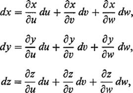
formal multiplication, using the relations

yields
![]()
(Exercise 5.20). These matters will be discussed more fully in Chapter V.
Exercises
5.1Let A be a bounded subset of ![]() k, with k < n. If f:
k, with k < n. If f: ![]() k →
k → ![]() n is a
n is a ![]() mapping, show that f(A) is negligible. Hint: Let Q be a cube in
mapping, show that f(A) is negligible. Hint: Let Q be a cube in ![]() k containing A, and
k containing A, and ![]() a partition of Q into Nk cubes with edgelength r/N, where r is the length of the edges of Q. Since f is
a partition of Q into Nk cubes with edgelength r/N, where r is the length of the edges of Q. Since f is ![]() on Q, there exists c such that
on Q, there exists c such that ![]() for all
for all ![]() . It follows that
. It follows that ![]() .
.
5.2Show that A is contented if and only if, given ε > 0, there exist contented sets A1 and A2 such that ![]() and v(A2 − A1) < ε.
and v(A2 − A1) < ε.
5.3(a) If ![]() is negligible and T:
is negligible and T: ![]() n →
n → ![]() n is a
n is a ![]() mapping, show that T(A) is negligible. Hint: Apply the fact that, given an interval Q containing A, there exists c > 0 such that
mapping, show that T(A) is negligible. Hint: Apply the fact that, given an interval Q containing A, there exists c > 0 such that ![]() T(x) − T(y)
T(x) − T(y)![]() < c
< c![]() x − y
x − y![]() for all
for all ![]() .
.
(b) If A is a contented set in ![]() n and T:
n and T: ![]() n →
n → ![]() n is a
n is a ![]() mapping which is
mapping which is ![]() -invertible on the interior of A, show that T(A) is contented. Hint: Show that
-invertible on the interior of A, show that T(A) is contented. Hint: Show that ![]() , and then apply (a).
, and then apply (a).
5.4Establish the conclusion of Theorem 5.5 under the hypothesis that Q is a contented set such that T is ![]() -invertible on the interior of Q. Hint: Let Q1, . . . , Qk be nonoverlapping intervals interior to Q, and
-invertible on the interior of Q. Hint: Let Q1, . . . , Qk be nonoverlapping intervals interior to Q, and ![]() . Then
. Then
![]()
by Theorem 5.5. Use the hint for Exercise 5.3(a) to show that v(T(K)) can be made arbitrarily small by making v(K) sufficiently small.
5.5Consider the n-dimensional solid ellipsoid
![]()
Note that E is the image of the unit ball Bn under the mapping T: ![]() n →
n → ![]() n defined by
n defined by
![]()
Apply Theorem 5.1 to show that v(E) = a1 a2 · · · anv(Bn). For example, the volume of the 3-dimensional ellipsoid ![]() is
is ![]() .
.
5.6Let R be the solid torus in ![]() 3 obtained by revolving the circle
3 obtained by revolving the circle ![]() , in the yz-plane, about the z-axis. Note that the mapping T:
, in the yz-plane, about the z-axis. Note that the mapping T: ![]() 3 →
3 → ![]() 3 defined by
3 defined by
maps the interval ![]() and
and ![]() onto this torus. Apply the change of variables formula to calculate its volume.
onto this torus. Apply the change of variables formula to calculate its volume.
5.7Use the substitution u = x − y, v = x + y to evaluate
![]()
where R is the first quadrant region bounded by the coordinate axes and the line x + y = 1.
5.8Calculate the volume of the region in ![]() 3 which is above the xy-plane, under the paraboloid z = x2 + y2, and inside the elliptic cylinder x2/9 + y2/4 = 1. Use elliptical coordinates x = 3r cos θ, y = 2r sin θ.
3 which is above the xy-plane, under the paraboloid z = x2 + y2, and inside the elliptic cylinder x2/9 + y2/4 = 1. Use elliptical coordinates x = 3r cos θ, y = 2r sin θ.
5.9Consider the solid elliptical rod bounded by the xy-plane, the plane z = αx + βy + h through the point (0, 0, h) on the positive z-axis, and the elliptical cylinder x2/a2 + y2/b2 = 1. Show that its volume is πabh (independent of α and β). Hint: Use elliptical coordinates x = ar cos θ, y = br sin θ.
5.10Use “double polar” coordinates defined by the equations
![]()
to show that the volume of the unit ball ![]() is
is ![]() .
.
5.11Use the transformation defined by
![]()
to evaluate
![]()
where R is the region in the first quadrant of the xy-plane which is bounded by the circles x2 + y2 = 6x, x2 + y2 = 4x, x2 + y2 = 8y, x2 + y2 = 2y.
5.12Use the transformation T from rθt-space to xyz-space, defined by
![]()
to find the volume of the region R which lies between the paraboloids z = x2 + y2 and z = 4(x2 + y2), and also between the planes z = 1 and z = 4.
5.13Consider a spherical ball of radius a centered at the origin, with a spherically symmetric density function d(x) = g(ρ).
(a)Use spherical coordinates to show that its mass is
![]()
(b)Show that the gravitational force exerted by this ball on a point mass m located at the point ξ = (0, 0, c), with c > a, is the same as if its mass were all concentrated at the origin, that is,
![]()
Hint:Because of symmetry considerations, you may assume that the force is directed toward 0, so only its z-component need be explicitly computed. In spherical coordinates (see Fig. 4.37),
![]()
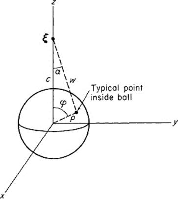
Figure 4.37
Change the second variable of integration from φ to w, using the relations
![]()
so 2w dw = 2ρc sin φ dφ, and w cos α + ρ cos φ = c (why ?).
5.14Consider now a spherical shell, centered at the origin and defined by ![]() , with a spherically symmetric density function. Show that this shell exerts no gravitational force on a point mass m located at the point (0, 0, c) inside it (that is, c < a). Hint: The computation is the same as in the previous problem, except for the limits of integration on ρ and w.
, with a spherically symmetric density function. Show that this shell exerts no gravitational force on a point mass m located at the point (0, 0, c) inside it (that is, c < a). Hint: The computation is the same as in the previous problem, except for the limits of integration on ρ and w.
5.15Volume of Revolution. Suppose g : [a, b] → ![]() is a positive-valued continuous function, and let
is a positive-valued continuous function, and let
![]()
Denote by C the set generated by revolving A about the z-axis (Fig. 4.38); that is,
![]()
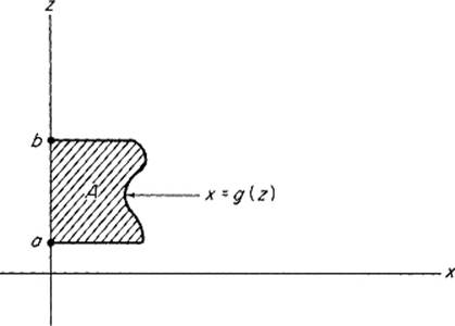
Figure 4.38
We wish to calculate v(C) = ∫c 1. Noting that C is the image of the contented set
![]()
under the cylindrical coordinates mapping T : ![]() 3 →
3 → ![]() 3 defined by T(r, θ, z) = (r cos θ, r sin θ, z), show that the change of variable and repeated integrals theorems apply to give
3 defined by T(r, θ, z) = (r cos θ, r sin θ, z), show that the change of variable and repeated integrals theorems apply to give
![]()
5.16Let A be a contented set in the right half xz-plane x > 0. Define ![]() , the x-coordinate of the centroid of A, by
, the x-coordinate of the centroid of A, by ![]() = [1/v(A)] ∫∫A x dx dz. If C is the set obtained by revolving A about the z-axis, that is,
= [1/v(A)] ∫∫A x dx dz. If C is the set obtained by revolving A about the z-axis, that is,
![]()
then Pappus' theorem asserts that
![]()
that is, that the volume of C is the volume of A multiplied by the distance traveled by the centroid of A. Note that C is the image under the cylindrical coordinates map of the set
![]()
Apply the change of variables and iterated integrals theorems to deduce Pappus' theorem.
The purpose of each of the next three problems is to verify the formulas
![]()
given in this section, for the volume αn of the unit n-ball ![]() .
.
5.17(a)Apply Cavalieri's principle and appropriate substitutions to obtain
Conclude that αn = 4αn−2 In In−1.
(b)Deduce from Exercise 1.8 that In In−1 = π/2n if ![]() . Hence
. Hence
![]()
(c)Use the recursion formula (#) to establish, by separate inductions on m, formulas (*), starting with α2 = π and α3 = 4π/3.
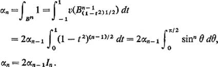
5.18In this problem we obtain the same recursion formula without using the formulas for I2n and I2n+1. Let
![]()
and ![]() : each
: each ![]() . Then
. Then ![]() . Let φ : B2 × Q →
. Let φ : B2 × Q → ![]() be the characteristic function of Bn. Then
be the characteristic function of Bn. Then
![]()
Note that, if ![]() is a fixed point, then φ, as a function of (x3, . . . , xn), is the characteristic function of
is a fixed point, then φ, as a function of (x3, . . . , xn), is the characteristic function of ![]() . Hence
. Hence
![]()
Now introduce polar coordinates in ![]() to show that
to show that
![]()
so that αn = (2π/n)αn−2 as before.
5.19The n-dimensional spherical coordinates mapping T: ![]() n →
n → ![]() n is defined by
n is defined by
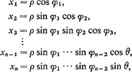
and maps the interval
![]()
onto the unit ball Bn.
(a)Prove by induction on n that
![]()
(b)Then
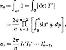
where ![]() . Now use the fact that
. Now use the fact that
![]()
(by Exercise 1.8) to establish formulas (*).
5.20Verify formulas (23) of this section.