Advanced Calculus of Several Variables (1973)

Part V. Line and Surface Integrals; Differential Forms and Stokes' Theorem

This chapter is an exposition of the machinery that is necessary for the statement, proof, and application of Stokes’ theorem. Stokes’ theorem is a multidimensional generalization of the fundamental theorem of (single-variable) calculus, and may accurately be called the “fundamental theorem of multi-variable calculus.” Among its numerous applications are the classical theorems of vector analysis (see Section 7) .

We will be concerned with the integration of appropriate kinds of functions over surfaces (or manifolds) in ⁿ. It turns out that the sort of “object,” which can be integrated over a smooth k-manifold in ⁿ, is what is called a differential k-form (defined in Section 5) . It happens that to every differential k-form α, there corresponds a differential (k + 1)-form dα, the differential of α, and Stokes' theorem is the formula

where V is a compact (k + 1)-dimensional manifold with nonempty boundary ∂V (a k-manifold). In the course of our discussion we will make clear the way in which this is a proper generalization of the fundamental theorem of calculus in the form

We start in Section 1 with the simplest case—integrals over curves in space, traditionally called “line integrals.” Section 2 is a leisurely treatment of the 2-dimensional special case of Stokes’ theorem, known as Green’s theorem; this will serve to prepare the student for the proof of the general Stokes' theorem in Section 6.

Section 3 includes the multilinear algebra that is needed for the subsequent discussions of surface area (Section 4) and differential forms (Section 5) . The student may prefer (at least in the first reading) to omit the proofs in Section 3 —only the definitions and statements of the theorems of this section are needed in the sequel.

Chapter 1. PATHLENGTH AND LINE INTEGRALS

In this section we generalize the familiar single-variable integral (on a closed interval in ) so as to obtain a type of integral that is associated with paths in ⁿ. By a path in ⁿ is meant a continuously differentiable function γ: [a, b] → ⁿ. The path γ : [a, b] → ⁿ is said to be smooth if γ′(t) ≠ 0 for all . The significance of the condition γ′(t) ≠ 0—that the direction of a path cannot change abruptly if its velocity vector never vanishes—is indicated by the following example.

Example 1 Consider the path γ = (γ₁, γ₂): → ² defined by

The image of γ is the graph y = x (Fig. 5.1) . The only “corner” occurs at the origin, which is the image of the single point t = 0 at which γ′(t) = 0.

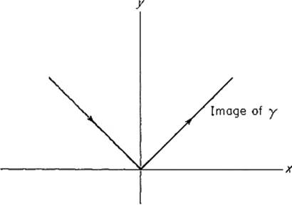
Figure 5.1

We discuss first the concept of length for paths. It is natural to approach the definition of the length s(γ) of the path γ : [a, b] → ⁿ by means of polygonal approximations to γ. Choose a partition of [a, b],

and recall that the mesh is the maximum length t_i − t_i−1 of a subinterval of . Then defines a polygonal approximation to γ, namely the polygonal arc from γ(a) to γ(b) having successive vertices γ(t₀), γ(t₁), . . . , γ(t_k) (Fig. 5.2) , and we regard the length

of this polygonal arc as an approximation to s(γ).

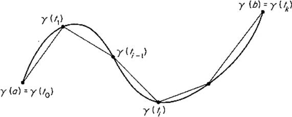
Figure 5.2

This motivates us to define the length s(γ) of the path γ : [a, b] → ⁿ by

provided that this limit exists, in the sense that, given > 0, there exists δ > 0 such that

It turns out that the limit in (1) may not exist if γ is only assumed to be continuous, but that it does exist if γ is a path, and moreover that there is then a pleasant means of computing it.

Theorem 1.1 If γ : [a, b] → ⁿ is a path, then s(γ) exists, and

REMARK If we think of a moving particle in ⁿ, whose position vector at time t is γ(t), then γ′(t) is its speed. Thus (2) simply asserts that the distance traveled by the particle is equal to the time integral of its speed—a result whose 1-dimensional case is probably familiar from elementary calculus.

PROOF It suffices to show that, given > 0, there exists δ > 0 such that

for every partition

of mesh less than δ. Recall that

where γ₁, . . . , γ_n are the component functions of γ.

An application of the mean value theorem to the function γ_r on the ith subinterval [t_i−1, t_i] yields a point such that

Consequently Eq. (3) becomes

If the points t_i¹, t_i², . . . , t_iⁿ just happened to all be the same point , then (4) would take the form

which is a Riemann sum for . This is the real reason for the validity of formula (2) ; the remainder of the proof consists in showing that the difference between the sum (4) and an actual Riemann sum is “negligible.”

For this purpose we introduce the auxiliary function F : I = [a, b]ⁿ → defined by

Notice that F(t, t, . . . , t) = γ′(t), and that F is continuous, and therefore uniformly continuous, on the n-dimensional interval I, since γ is a path. Consequently there exists a δ₁ > 0 such that

if each x_r − y_r < δ₁.

We now want to compare the approximation

with the Riemann sum

Since the points t_i¹, t_i², . . . , t_iⁿ all lie in the interval [t_i−1, t_i], whose length , it follows from (5) that

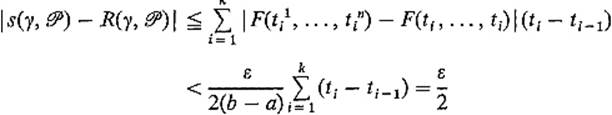
if < δ₁.

On the other hand, there exists (by Theorem IV.3.4) a δ₂ > 0 such that

if < δ₂.

If, finally, δ = min(δ₁, δ₂), then < δ implies that

as desired.

Example 2 Writing γ(t) = (x₁(t), . . . , x_n(t)), and using Leibniz notation, formula (2) becomes

Given a function f : [a, b] → , the graph of f is the image of the path γ : [a, b] → ² defined by γ(x) = (x, f(x)). Substituting x₁ = t = x and x₂ = y in the above formula with n = 2, we obtain the familiar formula

for the length of the graph of a function.

Having defined pathlength and established its existence for paths, the following question presents itself. Suppose that α : [a, b] → ⁿ and β : [c, d] → ⁿ are two paths that are “geometrically equivalent” in the sense that they have the same initial point α(a) = β(c), the same terminal point α(b) = β(d), and trace through the same intermediate points in the same order. Do α and β then have the same length, s(α) = s(β)?

Before providing the expected affirmative answer to this question, we must make precise the notion of equivalence of paths. We say that the path α : [a, b] → ⁿ is equivalent to the path β : [c, d] → ⁿ if and only if there exists a function

such that φ([a, b]) = [c, d], α = β φ, and φ′(t) > 0 for all (see Fig. 5.3) . The student should show that this relation is symmetric (if α is equivalent to β, then β is equivalent to α) and transitive (if α is equivalent to β, and βis equivalent to γ, then α is equivalent to γ), and is therefore an equivalence relation (Exercise 1.1) . He should also show that, if the paths α and β are equivalent, then α is smooth if and only if β is smooth (Exercise 1.2) .

The fact that s(α) = s(β) if α and β are equivalent is seen by taking f(x) ≡ 1 in the following theorem.

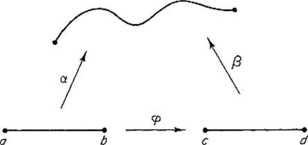
Figure 5.3

Theorem 1.2 Suppose that α : [a, b] → ⁿ and β : [c, d] → ⁿ are equivalent paths, and that f is a continuous real-valued function whose domain of definition in ⁿ contains the common image of α and β. Then

PROOF If φ : [a, b] → [c, d] is a function such that α = β φ and φ′(t) > 0 for all , then

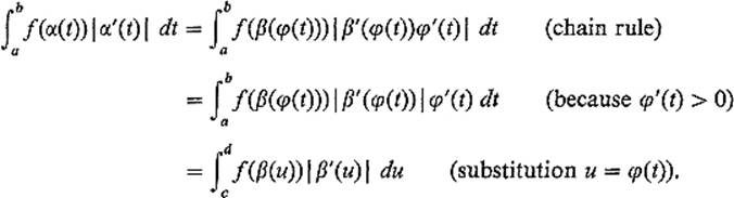
To provide a physical interpretation of integrals such as those of the previous theorem, let us think of a wire which coincides with the image of the path γ : [a, b] → ⁿ, and whose density at the point γ(t) is f(γ(t)). Given a partition = {a = t₀ < t₁ < · · · < t_k = b} of [a, b], the sum

may be regarded as an approximation to the mass of the wire. By an argument essentially identical to that of the proof of Theorem 1.1 , it can be proved that

Consequently this integral is taken as the definition of the mass of the wire.

If γ is a smooth path, the integral (6) can be interpreted as an integral with respect to pathlength. For this we need an equivalent unit-speed path, that is an equivalent smooth path such that ′(t) ≡ 1.

Proposition 1.3 Every smooth path γ : [a, b] → ⁿ is equivalent to a smooth unit-speed path.

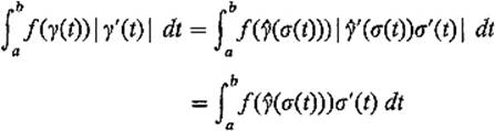
PROOF Write L = s(γ) for the length of γ, and define σ : [a, b] → [0, L] by

so σ(t) is simply the length of the path γ : [a, t] → ⁿ (Fig. 5.4) . Then from the fundamental theorem of calculus we see that σ is a function with

Therefore the inverse function τ : [0, L] → [a, b] exists, with

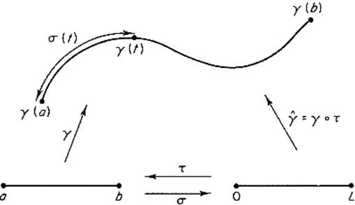
Figure 5.4

If : [0, L] → ⁿ is the equivalent smooth path defined by = γ τ, the chain rule gives

since σ′(t) = γ′(t).

With the notation of this proposition and its proof, we have

since ′(σ(t)) = 1 and σ′(t) > 0. Substituting s = σ(t), we then obtain

This result also follows immediately from (Theorem 1.2. ) Since (s) simply denotes that point whose “distance along the path” from the initial point γ(a) is s, Eq. (7) provides the promised integral with respect to pathlength.

It also serves to motivate the common abbreviation

Historically this notation resulted from the expression

for the length of the “infinitesimal” piece of path corresponding to the “infinitesimal” time interval [t, t + dt]. Later in this section we will provide the expression ds = γ′(t) dt with an actual mathematical meaning (in contrast to its “mythical” meaning here).

Now let γ : [a, b] → ⁿ be a smooth path, and think of γ(t) as the position vector of a particle moving in ⁿ under the influence of the continuous force field F : ⁿ → ⁿ [so F(γ(t)) is the force acting on the particle at time t]. We inquire as to the work W done by the force field in moving the particle along the path from γ(a) to γ(b). Let be the usual partition of [a, b]. If F were a constant force field, then the work done by F in moving the particle along the straight line segment from γ(t_i−1) to γ(t_i) would by definition be F · (γ(t_i) − γ(t_i−1)) (in the constant case, work is simply the product of force and distance). We therefore regard the sum

as an approximation to W. By an argument similar to the proof of Theorem 1.1 , it can be proved that

so we define the work done by the force field F in moving a particle along the path γ by

Rewriting (9) in terms of the unit tangent vector

at γ(t) (Fig. 5.5) , we obtain

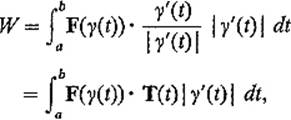
or

in the notation of (8) . Thus the work done by the force field is the integral with respect to pathlength of its “tangential component” F · T.

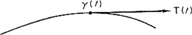
Figure 5.5

In terms of components, (9) becomes

or

in Leibniz notation. A classical abbreviation for this last formula is

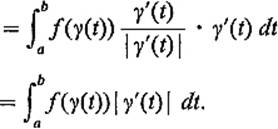
This type of integral, called a line integral (or curvilinear integral), can of course be defined without reference to the above discussion of work, and indeed line integrals have a much wider range of applications than this. Given a path γ : [a, b] → ⁿ and n continuous functions f₁, . . . , f_n whose domains of definition in ⁿ all contain the image of γ, the line integral ∫_γ f₁ dx₁ + · · · + f_n dx_n is defined by

Formally, we simply substitute x_i = γ_i(t), dx_i = γ_i′(t) dt into the left-hand side of (11) , and then integrate from a to b.

We now provide an interpretation of (11) whose viewpoint is basic to subsequent sections. By a (linear) differential form on the set is meant a mapping ω which associates with each point a linear function ω(x) : ⁿ → . Thus

where (ⁿ, ) is the vector space of all linear (real-valued) functions on ⁿ. We will frequently find it convenient to write

Recall that every linear function L : ⁿ → is of the form

where λ_i : ⁿ → is the ith projection function defined by

If we use the customary notation λ_i = dx_i, then (12) becomes

If L = ω(x) depends upon the point , then so do the coefficients a₁, . . . , a_n; this gives the following result.

Proposition 1.4 If ω is a differential form on , then there exist unique real-valued functions a₁, . . . , a_n on U such that

for each .

Thus we may regard a differential form as simply an “expression of the form” (13) , remembering that, for each , this expression denotes the linear function whose value at is

The differential form ω is said to be continuous (or differentiable, or ) provided that its coefficient functions a₁, . . . , a_n are continuous (or differentiable, or ).

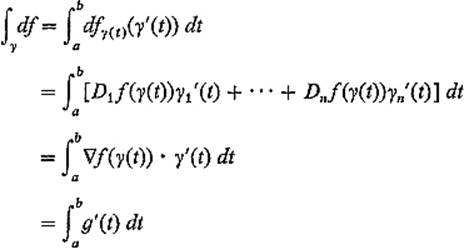
Now let ω be a continuous differential form on , and γ : [a, b] → U a path. We define the integral of ω over the path γ by

In other words, if ω = a₁ dx₁ + · · · + a_n dx_n, then

Note the agreement between this and formula (11) ; a line integral is simply the integral of the differential form appearing as its “integrand.”

Example 3 Let ω be the differential form defined on ² minus the origin by

If γ₁ : [0, 1] → ² − {0} is defined by γ₁(t) = (cos πt, sin πt), then the image of γ₁ is the upper half of the unit circle, and

If γ₂ : [0, 1] → ² − {0} is defined by γ₂(t) = (cos πt, − sin πt), then the image of γ₂ is the lower half of the unit circle (Fig. 5.6) , and

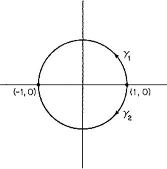
Figure 5.6

In a moment we will see the significance of the fact that .

Recall that, if f is a differentiable real-valued function on the open set , then its differential df_x at is the linear function on ⁿ defined by

Consequently we see that the differential of a differentiable function is a differential form

or

Example 4 Let U denote ² minus the nonnegative x-axis; that is, unless and y = 0. Let θ : U → be the polar angle function defined in the obvious way (Fig. 5.7) . In particular,

if x ≠ 0, so

Therefore

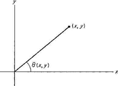
Figure 5.7

on U; the differential of θ agrees on its domain of definition U with the differential form ω of Example 3. Although

is defined on ² − {0}, it is clear that the angle function cannot be extended continuously to ² − {0}. As a consequence of the next theorem, we will see that ω is not the differential of any differentiable function that is defined on all of ² − {0}.

Recall the fundamental theorem of calculus in the form

Now f′(t) dt is simply the differential at t of f : → ; dt : → is the identity mapping. If γ : [a, b] → [a, b] is also the identity, then

and f(b) − f(a) = f(γ(b)) − f(γ(a)), so the fundamental theorem of calculus takes the form

The following theorem generalizes this formula; it is the “fundamental theorem of calculus for paths in ⁿ.”

Theorem 1.5 If f is a real-valued function on the open set , and γ : [a, b] → U is a path, then

PROOF Define g : [a, b] → by g = f γ. Then g′(t) = f(γ(t)) · γ′(t) by the chain rule, so

It is an immediate corollary to this theorem that, if the differential form ω on U is the differential of some function on the open set U, then the integral ∫_γ ω is independent of the path γ, to the extent that it depends only on the initial and terminal points of γ.

Corollary 1.6 If ω = df, where f is a function on U, and α and β are two paths in U with the same initial and terminal points, then

We now see that the result of Example 3 , where γ₁ and γ₂ were two different paths in ² − {0} from (1, 0) to (−1, 0), implies that the differential form

is not the differential of any function on ² − {0}. Despite this fact, it is customarily denoted by dθ, because its integral over a path γ measures the polar angle between the endpoints of γ.

Recall that, if F : U → ⁿ is a force field on and γ : [a, b] → ⁿ is a path in U, then the work done by the field F in transporting a particle along the path γ is defined by

where ω = F₁ dx₁ + · · · + F_n dx_n. Suppose now that the force field F is conservative (see Exercise II.1.3) , that is, there exists a function g : U → such that F = g. Since this means that ω = dg, Corollary 1.6 implies that Wdepends only on the initial and terminal points of γ, and in particular that

This is the statement that the work done by a conservative force field, in moving a particle from one point to another, is equal to the “difference in potential” of the two points.

We close this section with a discussion of the arclength form ds of an oriented curve in ⁿ. This will provide an explication of the notation of formulas (8) and (10) .

The set C in ⁿ is called a curve if and only if it is the image of a smooth path γ which is one-to-one. Any one-to-one smooth path which is equivalent to γ is then called a parametrization of C.

If , then

is a unit tangent vector to C at x (Fig. 5.8) , and it is easily verified that T(x) is independent of the chosen parametrization γ of C (Exercise 1.3) . Such a continuous mapping T : C → ⁿ, such that T(x) is a unit tangent vector to C at x, is called an orientation for C. An oriented curve is then a pair (C, T), where T is an orientation for C. However we will ordinarily abbreviate (C, −T) to C, and write − C for (C, −T), the same geometric curve with the opposite orientation.

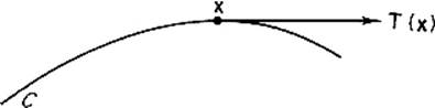
Figure 5.8

Given an oriented curve C in ⁿ, its arclength form ds is defined for by

Thus ds_x(v) is simply the component of v in the direction of the unit tangent vector T(x). It is clear that ds_x(v) is a linear function of , so ds is a differential form on C.

The following theorem expresses in terms of ds the earlier integrals of this section [compare with formulas (8) and (10) ].

Theorem 1.7 Let γ be a parametrization of the oriented curve (C, T), and let ds be the arclength form of C. If f : ⁿ → and F : ⁿ → ⁿ are continuous mappings, then

(so in particular s(γ) = ∫_γ ds), and

PROOF We verify (a), and leave the proof of (b) as an exercise. By routine application of the definitions, we obtain

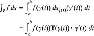
Finally notice that, if the differential form ω = F₁ dx₁ + · · · + F_n dx_n is defined on the oriented smooth curve (C, T) with parametrization γ, then

by Theorem 1.7(b) . Thus every integral of a differential form, over a parametrization of an oriented smooth curve, is an “arclength integral.”

Exercises

1.1Show that the relation of equivalence of paths in ⁿ is symmetric and transitive.

1.2If α and β are equivalent paths in ⁿ, and α is smooth, show that β is also smooth.

1.3Show that any two equivalent parametrizations of the smooth curve induce the same orientation of .

1.4If α and β are equivalent paths in ⁿ, and ω is a continuous differential form, show that ∫_α ω = ∫_β ω.

1.5If α : [0,1] → ⁿ is a path and ω is a continuous differential form, define β(t) = α(1 − t) for . Then show that ∫_αω = − ∫_βω.

1.6If α : [a, b] → ⁿ and β : [c, d] → ⁿ are smooth one-to-one paths with the same image, and α(a) = β(c), α(b) = β(d), show that α and β are equivalent.

1.7Show that the circumference of the ellipse x²/a² + y²/b² = 1 is

where denotes the standard “elliptic integral of the second kind.”

1.8(a)Given mappings define γ = T c. Show that

and conclude that the length of γ is

where

(b)Let be the spherical coordinates mapping given by

Let γ : [a, b] → ³ be a path on the unit sphere described by giving φ and θ as functions of t, that is, c(t) = (φ(t), θ(t)). Deduce from (a) that

1.9(a)Given mappings , define γ = F c. Show that

and conclude that the length of γ is

where g_ij = (∂F/∂u_i) • (∂F/∂u_j).

(b)Let be the cylindrical coordinates mapping given by

Let be a path described by giving r, θ, z as functions of t, that is,

Deduce from (a) that

1.10If F : ⁿ → ⁿ is a force field and γ : [a, b] → ⁿ a path, use the fact that F(γ(t)) = mγ′(t) to show that the work W done by this force field in moving a particle of mass m along the path γ from γ(a) to γ(b) is

where v(t) = γ′(t). Thus the work done by the field equals the increase in the kinetic energy of the particle.

1.11For each , let F(x, y) be a unit vector pointed toward the origin from (x, y). Calculate the work done by the force field F in moving a particle from (2a, 0) to (0, 0) along the top half of the circle (x − a)² + y² = a².

1.12Let dθ = (−y dx + x dy)/(x² + y²). Thinking of polar angles, explain why it seems “obvious” that ∫_γ dθ = 2π, where γ(t) = (a cos t, b sin t), . Accepting this fact, deduce from it that

1.13Let dθ = (−y dx + x dy)/(x² + y²) on ² − 0.

(a)If γ : [0, 1] → ² − 0 is defined by γ(t) = (cos 2kπt, sin 2kπt), where k is an integer, show that ∫_γdθ = 2kπ.

(b)If γ : [0, 1] → ² is a closed path (that is, γ(0) = γ(1)) whose image lies in the open first quadrant, conclude from Theorem 1.5 that ∫_γ dθ = 0.

1.14Let the differential form ω be defined on the open set , and suppose there exist continuous functions, f, g : → such that ω(x, y) = f(x) dx + g(y) dy if . Apply Theorem 1.5 to show that ∫_γ ω = 0 if γ is a closed path in U.

1.15Prove Theorem 1.7(b) . 8

1.16Let F : U → ⁿ be a continuous vector field on such that . If is a curve in U, and γ a parametrization of , show that

1.17If γ is a parametrization of the oriented curve with arclength form ds, show that ds_γ(t)(γ′(t)) = γ′(t), so

1.18Let γ(t) = (cos t, sin t) for be the standard parametrization of the unit circle in ². If

on ² − 0, calculate ∫_γ ω. Then explain carefully why your answer implies that there is no function f : ² − 0 → with df = ω.

1.19Let ω = y dx + x dy + 2z dz on ³. Write down by inspection a differentiable function f : ³ → such that df = ω. If γ: [a, b] → ³ is a path from (1, 0, 1) to (0, 1, −1), what is the value of ∫_γ ω?

1.20Let γ be a smooth parametrization of the curve in ², with unit tangent T and unit normal N defined by

and

Given a vector field F = (F₁, F₂) on ², let ω = −F₂ dx + F₁ dy, and then show that

1.21Let be an oriented curve in ⁿ, with unit tangent vector T = (t₁, . . . , t_n).

(a)Show that the definition [Eq. (16)] of the arclength form ds of C is equivalent to

(b)If the vector v is tangent to C, show that

(c)If F = (F₁, . . . , F_n) is a vector field, show that the 1-forms

agree on vectors that are tangent to C.