Advanced Calculus of Several Variables (1973)
Part V. Line and Surface Integrals; Differential Forms and Stokes' Theorem
Chapter 4. SURFACE AREA
In this section we investigate the concept of area for k-dimensional surfaces in ![]() n. A k-dimensional surface patch in
n. A k-dimensional surface patch in ![]() n is a
n is a ![]() mapping F : Q →
mapping F : Q → ![]() n, where Q is a k-dimensional interval (or rectangular parallelepiped) in
n, where Q is a k-dimensional interval (or rectangular parallelepiped) in ![]() k, which is one-to-one on the interior of Q.
k, which is one-to-one on the interior of Q.
Example 1 Let Q be the rectangle [0, 2π] × [0, π] in the θφ-plane ![]() 2, and F : Q →
2, and F : Q → ![]() 3 the surface patch defined by
3 the surface patch defined by
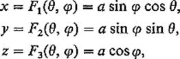
so a, θ, φ are the spherical coordinates of the point ![]() . Then the image of F is the sphere x2 + y2 + z2 = a2 of radius a (Fig. 5.22) . Notice that F is one-to-one on the interior of Q, but not on its boundary. The top edge of Q maps to the point (0, 0, −a), the bottom edge to (0, 0, a), and the image of each of the vertical edges is the semicircle
. Then the image of F is the sphere x2 + y2 + z2 = a2 of radius a (Fig. 5.22) . Notice that F is one-to-one on the interior of Q, but not on its boundary. The top edge of Q maps to the point (0, 0, −a), the bottom edge to (0, 0, a), and the image of each of the vertical edges is the semicircle ![]()
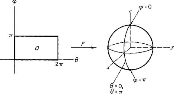
Figure 5.22
Example 2 Let Q be the square [0, 2π] × [0, 2π] in the θφ-plane ![]() 2, and F : Q →
2, and F : Q → ![]() 4 the surface patch defined by
4 the surface patch defined by
![]()
The image of F is the so-called “flat torus” ![]() in
in ![]() 4. Note that F is one-to-one on the interior of Q (why?), but not on its boundary [for instance, the four vertices of Q all map to the point
4. Note that F is one-to-one on the interior of Q (why?), but not on its boundary [for instance, the four vertices of Q all map to the point ![]() .
.
One might expect that the definition of surface area would parallel that of pathlength, so that the area of a surface would be defined as a limit of areas of appropriate inscribed polyhedral surfaces. These inscribed polyhedral surfaces for the surface patch F : Q → ![]() n could be obtained as follows (for k = 2; the process could be easily generalized to k > 2). Let
n could be obtained as follows (for k = 2; the process could be easily generalized to k > 2). Let ![]() = {σ1, . . . , σp} be a partition of the rectangle Q into small triangles (Fig. 5.23) . Then, for each i = 1, . . . , p, denote by τi that triangle in
= {σ1, . . . , σp} be a partition of the rectangle Q into small triangles (Fig. 5.23) . Then, for each i = 1, . . . , p, denote by τi that triangle in ![]() n whose three vertices are the images under F of the three vertices of σi. Our inscribed polyhedral approximation is then
n whose three vertices are the images under F of the three vertices of σi. Our inscribed polyhedral approximation is then
![]()
and its area is ![]() We would then define the area of the surface patch F by
We would then define the area of the surface patch F by
![]()
provided that this limit exists in the sense that, given ![]() > 0, there is a δ > 0 such that
> 0, there is a δ > 0 such that
![]()
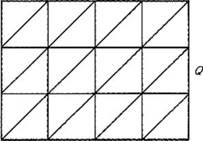
Figure 5.23
However it is a remarkable fact that the limit in (1) almost never exists if k > 1! The reason is that the triangles τi do not necessarily approximate the surface in the same manner that inscribed line segments approximate a smooth curve. For a partition of small mesh, the inscribed line segments to a curve have slopes approximately equal to those of the corresponding segments of the curve. However, in the case of a surface, the partition ![]() with small mesh can usually be chosen in such a way that each of the triangles τi is very nearly perpendicular to the surface. It turns out that, as a consequence, one can obtain inscribed polyhedra K
with small mesh can usually be chosen in such a way that each of the triangles τi is very nearly perpendicular to the surface. It turns out that, as a consequence, one can obtain inscribed polyhedra K![]() with
with ![]()
![]()
![]() arbitrarily small and a(K
arbitrarily small and a(K![]() ) arbitrarily large!
) arbitrarily large!
We must therefore adopt a slightly different approach to the definition of surface area. The basic idea is that the difficulties indicated in the previous paragraph can be avoided by the use of circumscribed polyhedral surfaces in place of inscribed ones. A circumscribed polyhedral surface is one consisting of triangles, each of which is tangent to the given surface at some point. Thus circumscribed triangles are automatically free of the fault (indicated above) of inscribed ones (which may be more nearly perpendicular to, than tangent to, the given surface).
Because circumscribed polyhedral surfaces are rather inconvenient to work with, we alter this latter approach somewhat, by replacing triangles with parallelepipeds, and by not requiring that they fit together so nicely as to actually form a continuous surface.
We start with a partition ![]() = {Q1, . . . , Qp} of the k-dimensional interval Q into small subintervals (Fig. 5.24) . It will simplify notational matters to assume that Q is a cube in
= {Q1, . . . , Qp} of the k-dimensional interval Q into small subintervals (Fig. 5.24) . It will simplify notational matters to assume that Q is a cube in ![]() k, so we may suppose that each subinterval Qi is a cube with edgelength h; its volume is then v(Qi) = hk.
k, so we may suppose that each subinterval Qi is a cube with edgelength h; its volume is then v(Qi) = hk.
Assuming that we already had an adequate definition of surface area, it would certainly be true that
![]()
where F ![]() Qi denotes the restriction of F to the subinterval Qi. We now approximate the sum on the right, replacing a(F
Qi denotes the restriction of F to the subinterval Qi. We now approximate the sum on the right, replacing a(F ![]() Qi) by a(dFqi(Qi)), the area of the
Qi) by a(dFqi(Qi)), the area of the
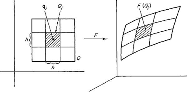
Figure 5.24
k-dimensional parallelepiped onto which Qi maps under the linear approximation dFqi to F, at an arbitrarily selected point ![]() (Fig. 5.25) . Then
(Fig. 5.25) . Then
![]()
where Pi = dFqi(Qi).
Now the parallelepiped Pi is spanned by the vectors
![]()
evaluated at the point ![]() . If Ai is the n × k matrix having these vectors as its column vectors, then
. If Ai is the n × k matrix having these vectors as its column vectors, then
![]()
by Theorem 3.10 . But it is easily verified that
![]()
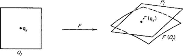
Figure 5.25
since the matrix F′ has column vectors ∂F/∂u1, . . . , ∂F/∂uk. Upon substitution of this into (2) , we obtain
![]()
Recognizing this as a Riemann sum, we finally define the (k-dimensional) surface area a(F) of the surface patch F : Q → ![]() n by
n by
![]()
Example 3If F is the spherical coordinates mapping of Example 1 , mapping the rectangle ![]() onto the sphere of radius a in
onto the sphere of radius a in ![]() 3, then a routine computation yields
3, then a routine computation yields
![]()
so (3) gives
![]()
as expected.
Example 4If F : [a, b] → ![]() n is a
n is a ![]() path, then
path, then
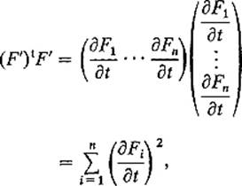
so we recover from (3) the familiar formula for pathlength.
Example 5We now consider 2-dimensional surfaces in ![]() n. Let φ : Q →
n. Let φ : Q → ![]() n be a 2-dimensional surface patch, where Q is a rectangle in the uv-plane. Then
n be a 2-dimensional surface patch, where Q is a rectangle in the uv-plane. Then
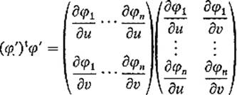
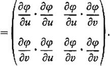
Equation (3) therefore yields
![]()
where
![]()
If we apply Corollary 3.8 to Eq. (3) , we obtain
![]()
where the notation [i] signifies (as usual) summation over all increasing k-tuples i = (i1, . . . , ik), and Fi′ is the k × k matrix whose rth row is the irth row of the derivative matrix F′ = (∂Fi/∂uj). With the Jacobian determinant notation
![]()
Eq. (5) becomes
![]()
We may alternatively explain the [i] notation with the statement that the summation is over all k × k submatrices of the n × k derivative matrix F′.
In the case k = 2, n = 3 of a 2-dimensional surface patch F in ![]() 3, given by
3, given by
![]()
(6) reduces to
![]()
Example 6We consider the graph in ![]() n of a
n of a ![]() function f : Q →
function f : Q → ![]() , where Q is an interval in
, where Q is an interval in ![]() n−1. This graph is the image in
n−1. This graph is the image in ![]() n of the surface patch F : Q →
n of the surface patch F : Q → ![]() n defined by
n defined by
![]()
The derivative matrix of F is
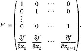
We want to apply (6) to compute a(F). First note that
![]()
If i < n, then
![]()
is the determinant of the (n − 1) × (n − 1) matrix Ai which is obtained from F′ upon deletion of its ith row. The elements of the ith column of Ai are all zero, except for the last one, which is ∂f/∂xi. Since the cofactor of ∂f/∂xi in Ai is the (n − 2) × (n − 2) identity matrix, expansion by minors along the ith column of Ai gives
![]()
for i < n. Substitution of (8) and (9) into (6) gives
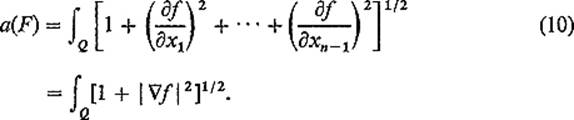
In the case n = 3, where we are considering a graph z = f(x, y) in ![]() 3 over
3 over ![]() and F(x, y) = (x, y, f(x, y)), formula (10) reduces to
and F(x, y) = (x, y, f(x, y)), formula (10) reduces to
![]()
This, together with (4) and (7) above, are the formulas for surface area in ![]() 3 that are often seen in introductory texts.
3 that are often seen in introductory texts.
Example 7 We now apply formula (10) to calculate the (n − 1)-dimensional area of the sphere ![]() of radius r, centered at the origin in
of radius r, centered at the origin in ![]() n. The upper hemisphere of
n. The upper hemisphere of ![]() is the graph in
is the graph in ![]() n of the function
n of the function
![]()
defined for ![]() f is continuous on
f is continuous on ![]() and
and ![]() on int
on int ![]() where
where
![]()
so
![]()
and therefore
![]()
Hence we are motivated by (10) to define a![]() by
by
![]()
This is an improper integral, but we proceed with impunity to compute it. In order to “legalize” our calculation, one would have to replace integrals over ![]() with integrals over
with integrals over ![]() , and then take limits as
, and then take limits as ![]() → 0.
→ 0.
If ![]() is defined by T(u) = ru, then
is defined by T(u) = ru, then ![]() and det T′ = rn−1, so the change of variables theorem gives
and det T′ = rn−1, so the change of variables theorem gives
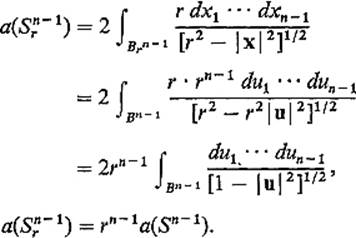
Thus the area of an (n − 1)-dimensional sphere is proportional to the (n − 1)th power of its radius (as one would expect).
Henceforth we write
![]()
for the area of the unit (n − 1)-sphere ![]() . By an application of Fubini's theorem, we obtain (see Fig. 5.26)
. By an application of Fubini's theorem, we obtain (see Fig. 5.26)
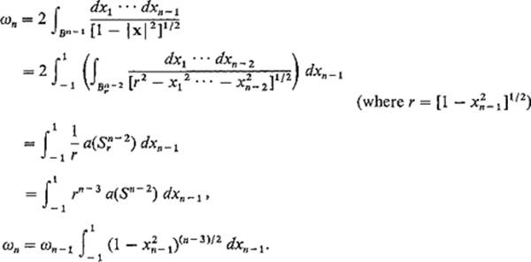
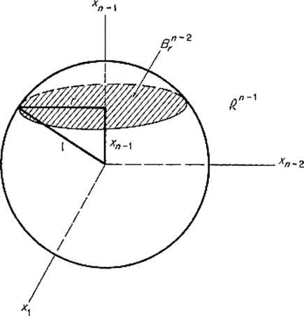
Figure 5.26
With the substitution xn−1 = cos θ we finally obtain
![]()
where
![]()
Since Ik Ik−1 = π/2k by Exercise IV.5.17 , it follows that
![]()
if ![]() In Exercise 4.10 this recursion relation is used to show that
In Exercise 4.10 this recursion relation is used to show that
![]()
for all ![]()
In the previous example we defined a(Sn−1) in terms of a particular parametrization of the upper hemisphere of Sn−1. There is a valid objection to this procedure—the area of a manifold in ![]() n should be defined in an intrinsic manner which is independent of any particular parametrization of it (or of part of it). We now proceed to give such a definition.
n should be defined in an intrinsic manner which is independent of any particular parametrization of it (or of part of it). We now proceed to give such a definition.
First we need to discuss k-cells in ![]() n. The set
n. The set ![]() is called a (smooth) k-cell if it is the image of the unit cube
is called a (smooth) k-cell if it is the image of the unit cube ![]() under a one-to-one
under a one-to-one ![]() mapping φ : U →
mapping φ : U → ![]() n which is defined on a neighborhood U of Ik, with the derivative matrix φ′(u) having maximal rank k for each
n which is defined on a neighborhood U of Ik, with the derivative matrix φ′(u) having maximal rank k for each ![]() (Fig. 5.27) . The mapping
(Fig. 5.27) . The mapping
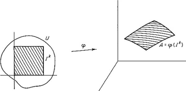
Figure 5.27
φ (restricted to Ik) is then called a parametrization of A. The following theorem shows that the area of a k-cell ![]() is well defined. That is, if φ and
is well defined. That is, if φ and ![]() are two parametrizations of the k-cell A, then a(φ) = a(
are two parametrizations of the k-cell A, then a(φ) = a(![]() ), so their common value may be denoted by a(A).
), so their common value may be denoted by a(A).
Theorem 4.1 If φ and ![]() are two parametrizations of the k-cell
are two parametrizations of the k-cell ![]() , then
, then
![]()
PROOF Since φ′(u) has rank k, the differential dφu maps ![]() k one-to-one onto the tangent k-plane to A at φ(u), and the same is true of d
k one-to-one onto the tangent k-plane to A at φ(u), and the same is true of d![]() u. If
u. If
![]()
is defined by T = ![]() −1
−1 ![]() φ, it follows that T is a
φ, it follows that T is a ![]() one-to-one mapping with det T′(u) ≠ 0 for all
one-to-one mapping with det T′(u) ≠ 0 for all ![]() so, by the inverse function theorem, T is
so, by the inverse function theorem, T is ![]() -invertible.
-invertible.
Since φ = T ![]()
![]() , the chain rule gives
, the chain rule gives
![]()
so
![]()
Consequently the change of variables theorem gives
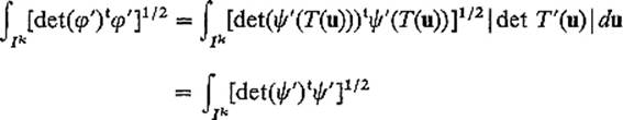
as desired. ![]()
If M is a compact smooth k-manifold in ![]() n, then M is the union of a finite number of nonoverlapping k-cells. That is, there exist k-cells A1, . . . , Ar in
n, then M is the union of a finite number of nonoverlapping k-cells. That is, there exist k-cells A1, . . . , Ar in ![]() n such that
n such that ![]() and int
and int ![]() if i ≠ j. Such a collection {A1, . . . , Ar} is called a paving of M. The proof that every compact smooth manifold in
if i ≠ j. Such a collection {A1, . . . , Ar} is called a paving of M. The proof that every compact smooth manifold in ![]() n is payable (that is, has a paving) is very difficult, and will not be included here. However, if we assume this fact, we can define the (k-dimensional) area a(M) of M by
n is payable (that is, has a paving) is very difficult, and will not be included here. However, if we assume this fact, we can define the (k-dimensional) area a(M) of M by
![]()
Of course it must be verified that a(M) is thereby well defined. That is, if {B1, . . . , Bs} is a second paving of M, then
![]()
The proof is outlined in Exercise 4.13 .
Example 8 We now employ the above definition, of the area of a smooth manifold in ![]() n, to give a second computation of ωn = a(Sn−1). Let {A1, . . . , Ak} be a paving of Sn−1. Let φ : In−1 → Ai be a parametrization of Ai. Then, given
n, to give a second computation of ωn = a(Sn−1). Let {A1, . . . , Ak} be a paving of Sn−1. Let φ : In−1 → Ai be a parametrization of Ai. Then, given ![]() > 0, define φ : In−1 × [
> 0, define φ : In−1 × [![]() , 1] →
, 1] → ![]() n by
n by
![]()
Denote by Bi the image of φ (see Fig. 5.28) . Then
![]()
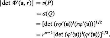
by the change of variables theorem. Now ![]() det φ′(u, r) is the volume of the n-dimensional parallelepiped P which is spanned by the vectors
det φ′(u, r) is the volume of the n-dimensional parallelepiped P which is spanned by the vectors
![]()
[evaluated at (u, r)]. But
![]()
is a unit vector which is orthogonal to each of the vectors
![]()
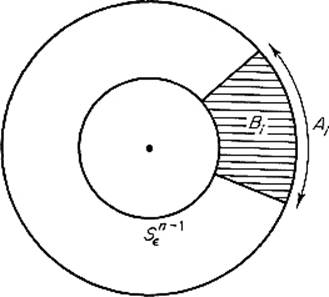
Figure 5.28
since the vectors r ∂φ/∂u1, . . . , r ∂φ/∂un−1 are tangent to Sn−1. If Q is the (n − 1)-dimensional parallelepiped which is spanned by these n − 1 vectors, it follows that v(P) = a(Q). Consequently we have
Substituting this into (11) , and applying Fubini's theorem, we obtain
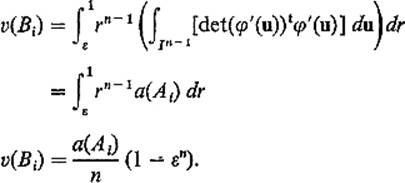
Summing from i = 1 to i = k, we then obtain
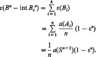
Finally taking the limit as ![]() → 0, we obtain
→ 0, we obtain
![]()
or
![]()
Consulting Exercise IV.6.3 for the value of v(Bn), this gives the value for a(Sn−1) listed at the end of Example 7 .
Exercises
4.1Consider the cylinder ![]() in
in ![]() 3. Regarding it as the image of a surface patch defined on the rectangle [0, 2π] × [0, h] in the θz-plane, apply formula (3) or (4) to show that its area is 2πah.
3. Regarding it as the image of a surface patch defined on the rectangle [0, 2π] × [0, h] in the θz-plane, apply formula (3) or (4) to show that its area is 2πah.
4.2Calculate the area of the cone ![]() noting that it is the image of a surface patch defined on the rectangle [0, 1] × [0, 2π] in the rθ-plane.
noting that it is the image of a surface patch defined on the rectangle [0, 1] × [0, 2π] in the rθ-plane.
4.3Let T be the torus obtained by rotating the circle z2 + (y − a)2 = b2 about the z-axis. Then T is the image of the square ![]() in the φθ-plane under the mapping F :
in the φθ-plane under the mapping F : ![]() 2 →
2 → ![]() 3 defined by
3 defined by
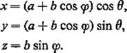
Calculate its area (answer = 4π2ab).
4.4Show that the area of the “flat torus” ![]() of Example 2 , is (2π)2. Generalize this computation to show that the area, of the “n-dimensional torus”
of Example 2 , is (2π)2. Generalize this computation to show that the area, of the “n-dimensional torus” ![]()
4.5Consider the generalized torus ![]() Use spherical coordinates in each factor to define a surface patch whose image is S2 × S2. Then compute its area.
Use spherical coordinates in each factor to define a surface patch whose image is S2 × S2. Then compute its area.
4.6Let C be a curve in the yz-plane described by y = α(t), z = β(t) for ![]() The surface swept out by revolving C around the z-axis is the image of the surface patch φ : [0, 2φ] × [a, b] →
The surface swept out by revolving C around the z-axis is the image of the surface patch φ : [0, 2φ] × [a, b] → ![]() 3 defined by
3 defined by
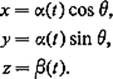
Show that a(φ) equals the length of C times the distance traveled by its centroid, that is,
![]()
4.7Let γ(s) = (α(s), β(s)) be a unit-speed curve in the xy-plane, so (α′)2 + (β′)2 = 1. The “tube surface” with radius r and center-line γ is the image of φ : [0, L] × [0, 2π] → ![]() 3, where φ is given by
3, where φ is given by
Show that a(φ) = 2πrL.
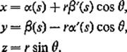
4.8This exercise gives an n-dimensional generalization of “Pappus' theorem for surface area” (Exercise 4.6) . Let φ : Q → ![]() n−1 be a k-dimensional surface patch in
n−1 be a k-dimensional surface patch in ![]() n−1, such that
n−1, such that ![]() for all
for all ![]() . The (k + 1)-dimensional surface patch
. The (k + 1)-dimensional surface patch
![]()
obtained by “revolving φ about the coordinate hyperplane ![]() n−2,” is defined by
n−2,” is defined by
![]()
for ![]() . Write down the matrix
. Write down the matrix ![]() and conclude from inspection of it that
and conclude from inspection of it that
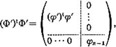
so
![]()
Deduce from this that
![]()
where ![]() n−1 is the (n − 1)th coordinate of the centroid of φ, defined by
n−1 is the (n − 1)th coordinate of the centroid of φ, defined by
![]()
4.9Let T : ![]() n →
n → ![]() n be the linear mapping defined by T(x) = bx. If φ : Q →
n be the linear mapping defined by T(x) = bx. If φ : Q → ![]() n is a k-dimensional surface patch in
n is a k-dimensional surface patch in ![]() n, prove that a(T
n, prove that a(T ![]() φ) = bka(φ).
φ) = bka(φ).
4.10Starting with ω2 = 2π and ω3 = 4π, use the recursion formula
![]()
of Example 7 , to establish, by separate inductions on m, the formulas
![]()
and
![]()
for ωn = a(Sn−1). Consulting Exercise IV.6.2, deduce that
![]()
for all ![]()
4.11Use the n-dimensional spherical coordinates of Exercise IV.5.19 to define an (n − 1)dimensional surface patch whose image is Sn−1. Then show that its area is given by the formula of the previous exercise.
4.12This exercise is a generalization of Example 8 . Let M be a smooth compact (n − 1)-manifold in ![]() n, and φ : M × [a, b] →
n, and φ : M × [a, b] → ![]() n a one-to-one
n a one-to-one ![]() mapping. Write Mt = φ(M × {t}). Suppose that, for each
mapping. Write Mt = φ(M × {t}). Suppose that, for each ![]() the curve γx(t) = φ(x, t) is a unit-speed curve which is orthogonal to each of the manifolds Mt. If A = φ(M × [a, b]), prove that
the curve γx(t) = φ(x, t) is a unit-speed curve which is orthogonal to each of the manifolds Mt. If A = φ(M × [a, b]), prove that
![]()
4.13Let M be a smooth k-manifold in ![]() n, and suppose {A1, . . . , Ar} and {B1, . . . , Bs} are two collections of nonoverlapping k-cells such that
n, and suppose {A1, . . . , Ar} and {B1, . . . , Bs} are two collections of nonoverlapping k-cells such that
![]()
Then prove that
![]()
Hint: Let φi and ![]() j be parametrizations of Ai and Bj, respectively. Define
j be parametrizations of Ai and Bj, respectively. Define
![]()
Then
![]()
while
![]()
Show by the method of proof of Theorem 4.1 , using Exercises IV.5.3 and IV.5.4 , that corresponding terms in the right-hand sums are equal.